import polars as pl
from plotnine import *
import datetimeA Century of Screams
area
contest
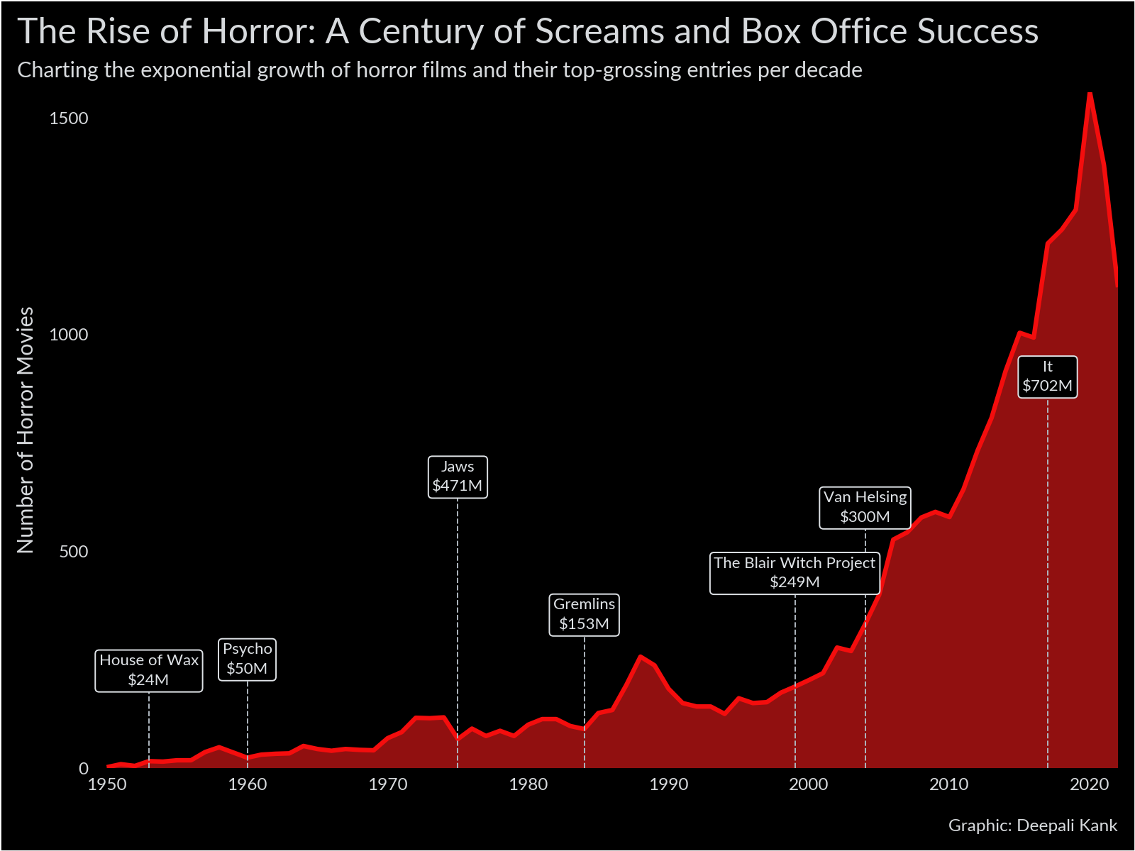
We analyze the trends and box office success of horror movies over the years. We will explore the data to understand the rise of horror films and identify the top-grossing english movies per decade.
Read the movie data
movies = pl.read_csv(
    "data/english_horror_movies.csv",
    schema_overrides={"release_date": pl.Date},
).with_columns(
    year=pl.col("release_date").dt.year(),
    revenue_millions=(pl.col("revenue") / 1_000_000).round(0).cast(int),
)
movies.head()
shape: (5, 13)
| title | release_date | revenue | popularity | vote_count | vote_average | budget | runtime | adult | genre_names | collection_name | year | revenue_millions |
|---|---|---|---|---|---|---|---|---|---|---|---|---|
| str | date | i64 | f64 | i64 | f64 | i64 | i64 | bool | str | str | i32 | i64 |
| "Orphan: First Kill" | 2022-07-27 | 9572765 | 5088.584 | 902 | 6.9 | 0 | 99 | false | "Horror, Thriller" | "Orphan Collection" | 2022 | 10 |
| "Beast" | 2022-08-11 | 56000000 | 2172.338 | 584 | 7.1 | 0 | 93 | false | "Adventure, Drama, Horror" | "NA" | 2022 | 56 |
| "Smile" | 2022-09-23 | 45000000 | 1863.628 | 114 | 6.8 | 17000000 | 115 | false | "Horror, Mystery, Thriller" | "NA" | 2022 | 45 |
| "The Black Phone" | 2022-06-22 | 161000000 | 1071.398 | 2736 | 7.9 | 18800000 | 103 | false | "Horror, Thriller" | "NA" | 2022 | 161 |
| "Jeepers Creepers: Reborn" | 2022-09-15 | 2892594 | 821.605 | 125 | 5.8 | 20000000 | 88 | false | "Horror, Mystery, Thriller" | "Jeepers Creepers Collection" | 2022 | 3 |
Get a tally of the movies per year
movies_per_year = movies.group_by("year").len("count").sort("year")
movies_per_year.head()
shape: (5, 2)
| year | count |
|---|---|
| i32 | u32 |
| 1950 | 2 |
| 1951 | 9 |
| 1952 | 5 |
| 1953 | 16 |
| 1954 | 15 |
Calculate the top movies per decade
top_movies_per_decade = movies.with_columns(
    decade=(pl.col("year") // 10 ) * 10
).filter(
    pl.col("year") < 2020,
).sort(
    "revenue_millions",
    descending=True
).group_by(
    "decade",
).first(
).select(
    "title", "year", "decade", "revenue_millions"
).sort(
    "decade"
).with_columns(
   label=pl.col("title") + "\n$" + pl.col("revenue_millions").cast(str) + "M",
    # Keep the labels in order of revenue, and adjust them
    # vertically so that they do not overlap
    label_position=pl.when(
        pl.col("title") == "Van Helsing"
    ).then(
        pl.col("revenue_millions") + 300
    ).otherwise(
        pl.col("revenue_millions") + 200
    ),
)
top_movies_per_decade
shape: (7, 6)
| title | year | decade | revenue_millions | label | label_position |
|---|---|---|---|---|---|
| str | i32 | i32 | i64 | str | i64 |
| "House of Wax" | 1953 | 1950 | 24 | "House of Wax $24M" | 224 |
| "Psycho" | 1960 | 1960 | 50 | "Psycho $50M" | 250 |
| "Jaws" | 1975 | 1970 | 471 | "Jaws $471M" | 671 |
| "Gremlins" | 1984 | 1980 | 153 | "Gremlins $153M" | 353 |
| "The Blair Witch Project" | 1999 | 1990 | 249 | "The Blair Witch Project $249M" | 449 |
| "Van Helsing" | 2004 | 2000 | 300 | "Van Helsing $300M" | 600 |
| "It" | 2017 | 2010 | 702 | "It $702M" | 902 |
For the contest submission, Deepali used Corbel, a proprietary font that matches well with the theme of the plot. Since Corbel isn’t freely available, we instead use Lato which is an open-source font that is likely available most systems.
body_font = "Lato"Plot
(
    ggplot(movies_per_year, aes("year", "count"))
    + geom_area(fill="#911010")
    + geom_line(color="#F40D0D", size=1.3)
    + geom_segment(
        aes(x="year", xend="year", y=0, yend="label_position"),
        top_movies_per_decade,
        color="#ADB5BD",
        linetype="dashed",
        size=0.4,
    )
    + geom_label(
        aes(
            "year",
            "label_position",
            label="label"
        ),
        top_movies_per_decade,
        color="#DEE2E6",
        fill="black",
        size=8,
        lineheight=1.5,
    )
    + labs(
        y="Number of Horror Movies",
        title="The Rise of Horror: A Century of Screams and Box Office Success",
        subtitle="Charting the exponential growth of horror films and their top-grossing entries per decade",
        caption="Graphic: Deepali Kank"
    )
    + scale_x_continuous(breaks=range(1950, 2022, 10), expand=(0, 1, 0, 0))
    + scale_y_continuous(expand=(0, 0))
    + theme(
        figure_size=(8, 6),
        plot_margin=0.015,
        panel_background=element_rect(fill="black"),
        plot_background=element_rect(fill="black"),
        plot_title=element_text(size=18),
        text=element_text(color="#D7DADD", family=body_font),
        panel_grid=element_blank(),
        panel_grid_major_x=element_blank(),
        axis_ticks=element_blank(),
        plot_title_position="plot",
        axis_title_x=element_blank(),
        axis_text_x=element_text(margin={"t": 5, "units": "pt"}),
        plot_caption=element_text(margin={"t": 10, "units": "pt"}),
    )
)
Where to find Deepali Kank: