after_stat

In [1]:

import pandas as pd
import numpy as np

from plotnine import ggplot, aes, after_stat, geom_bar, labs

geom_bar uses stat_count which by default maps the y aesthetic to the count which is the number of observations at a position.

In [2]:

df = pd.DataFrame({
    "var1": [1, 2, 2, 3, 3, 3, 4, 4, 4, 4, 5, 5, 5, 5, 5]
})

(
    ggplot(df, aes("var1"))
    + geom_bar()
)

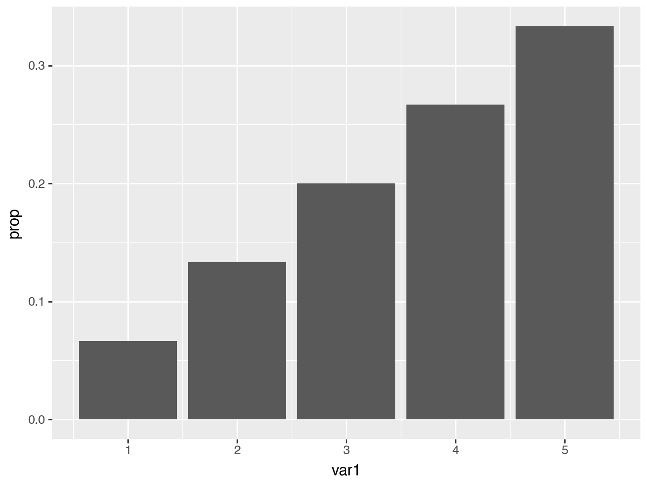
Using the after_stat function, we can instead map to the prop which is the ratio of points in the panel at a position.

In [3]:

(
    ggplot(df, aes("var1"))
    + geom_bar(aes(y=after_stat("prop")))  # default is after_stat('count')
)

With after_stat you can used the variables calculated by the stat in expressions. For example we use the count to calculated the prop.

In [4]:

(
    ggplot(df, aes("var1"))
    + geom_bar(aes(y=after_stat("count / np.sum(count)")))
    + labs(y="prop")
)

By default geom_bar uses stat_count to compute a frequency table with the x aesthetic as the key column. As a result, any mapping (other than the x aesthetic is lost) to a continuous variable is lost (if you have a classroom and you compute a frequency table of the gender, you lose any other information like height of students).

For example, below fill='var1' has no effect, but the var1 variable has not been lost it has been turned into x aesthetic.

In [5]:

(ggplot(df, aes("var1")) + geom_bar(aes(fill="var1")))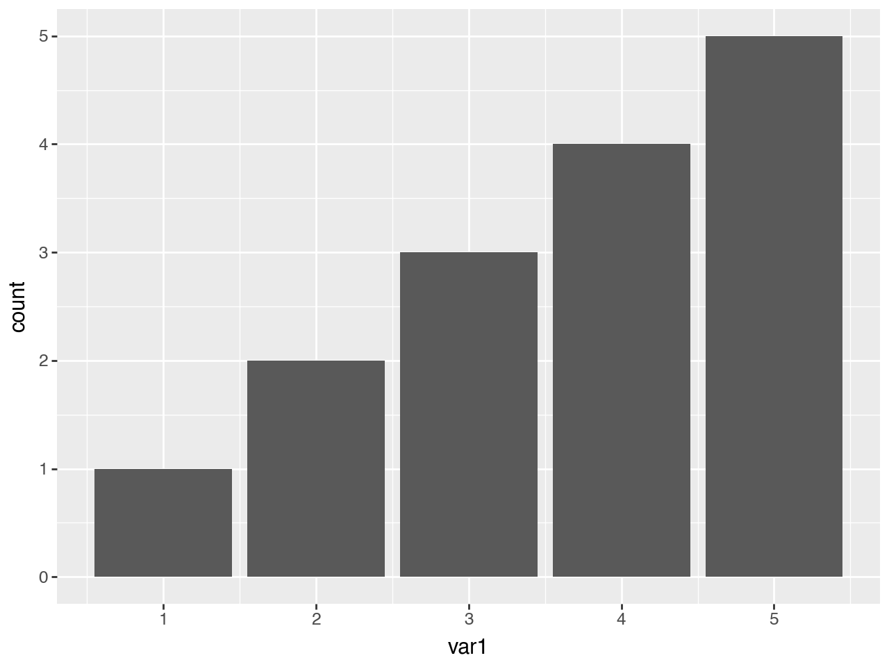

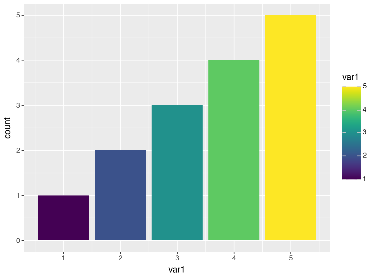
We use after_stat to map fill to the x aesthetic after it has been computed.

In [6]:

(
    ggplot(df, aes("var1"))
    + geom_bar(aes(fill=after_stat("x")))
    + labs(fill="var1")
)