Facet wrap

from plotnine import ggplot, aes, geom_point, labs, facet_wrap, theme
from plotnine.data import mpg

facet_wrap() creates a collection of plots (facets), where each plot is differentiated by the faceting variable. These plots are wrapped into a certain number of columns or rows as specified by the user.

mpg.head()

	manufacturer	model	displ	year	cyl	trans	drv	cty	hwy	fl	class
0	audi	a4	1.8	1999	4	auto(l5)	f	18	29	p	compact
1	audi	a4	1.8	1999	4	manual(m5)	f	21	29	p	compact
2	audi	a4	2.0	2008	4	manual(m6)	f	20	31	p	compact
3	audi	a4	2.0	2008	4	auto(av)	f	21	30	p	compact
4	audi	a4	2.8	1999	6	auto(l5)	f	16	26	p	compact

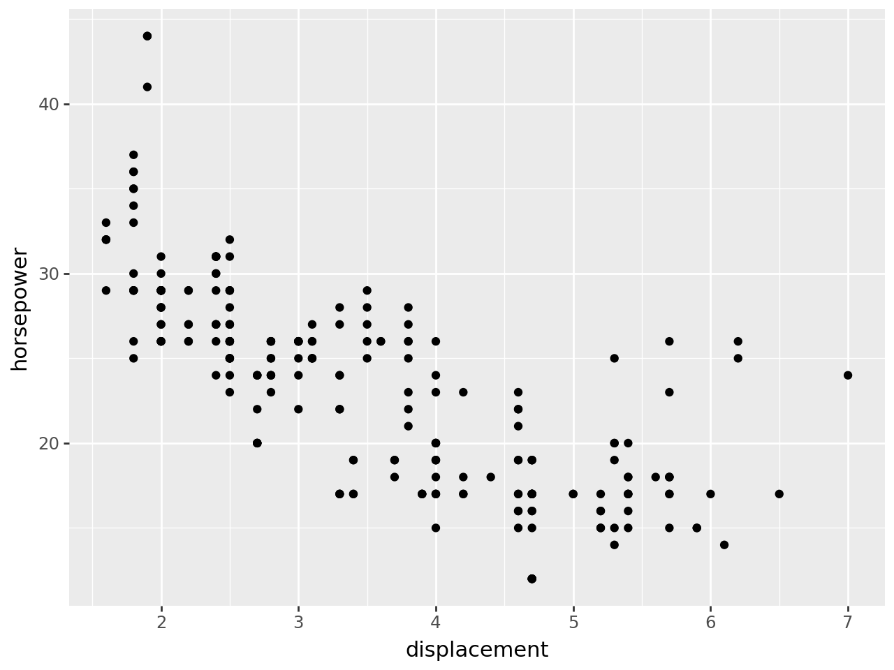
Basic scatter plot:

(
    ggplot(mpg, aes(x="displ", y="hwy"))
    + geom_point()
    + labs(x="displacement", y="horsepower")
)

Facet a discrete variable using facet_wrap():

(
    ggplot(mpg, aes(x="displ", y="hwy"))
    + geom_point()
    + facet_wrap("class")
    + labs(x="displacement", y="horsepower")
)

Control the number of rows and columns with the options nrow and ncol:

# Selecting the number of columns to display
(
    ggplot(mpg, aes(x="displ", y="hwy"))
    + geom_point()
    + facet_wrap(
        "class",
        ncol=4,  # change the number of columns
    )
    + labs(x="displacement", y="horsepower")
)

# Selecting the number of rows to display

(
    ggplot(mpg, aes(x="displ", y="hwy"))
    + geom_point()
    + facet_wrap(
        "class",
        nrow=4,  # change the number of columns
    )
    + labs(x="displacement", y="horsepower")
)

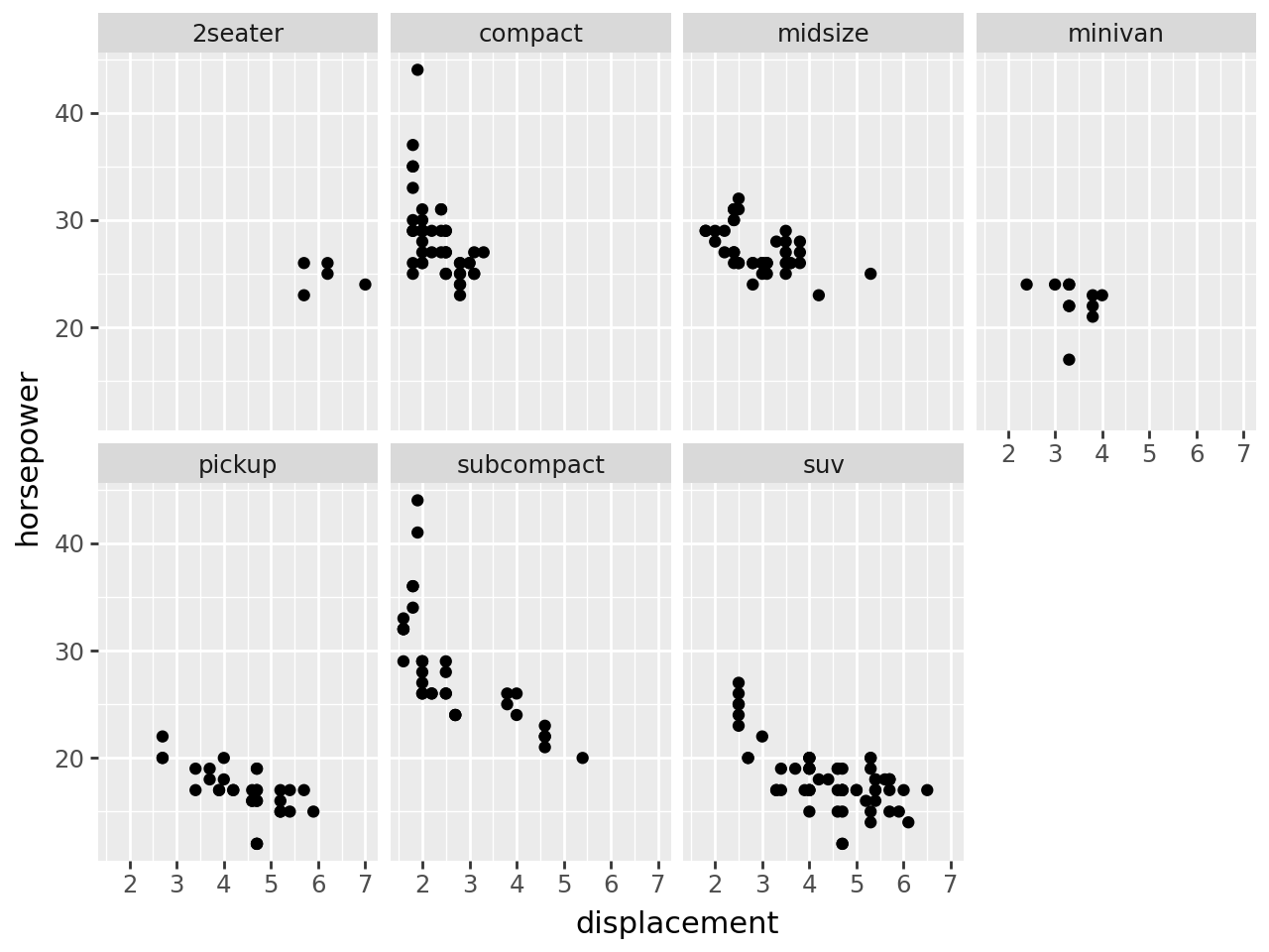
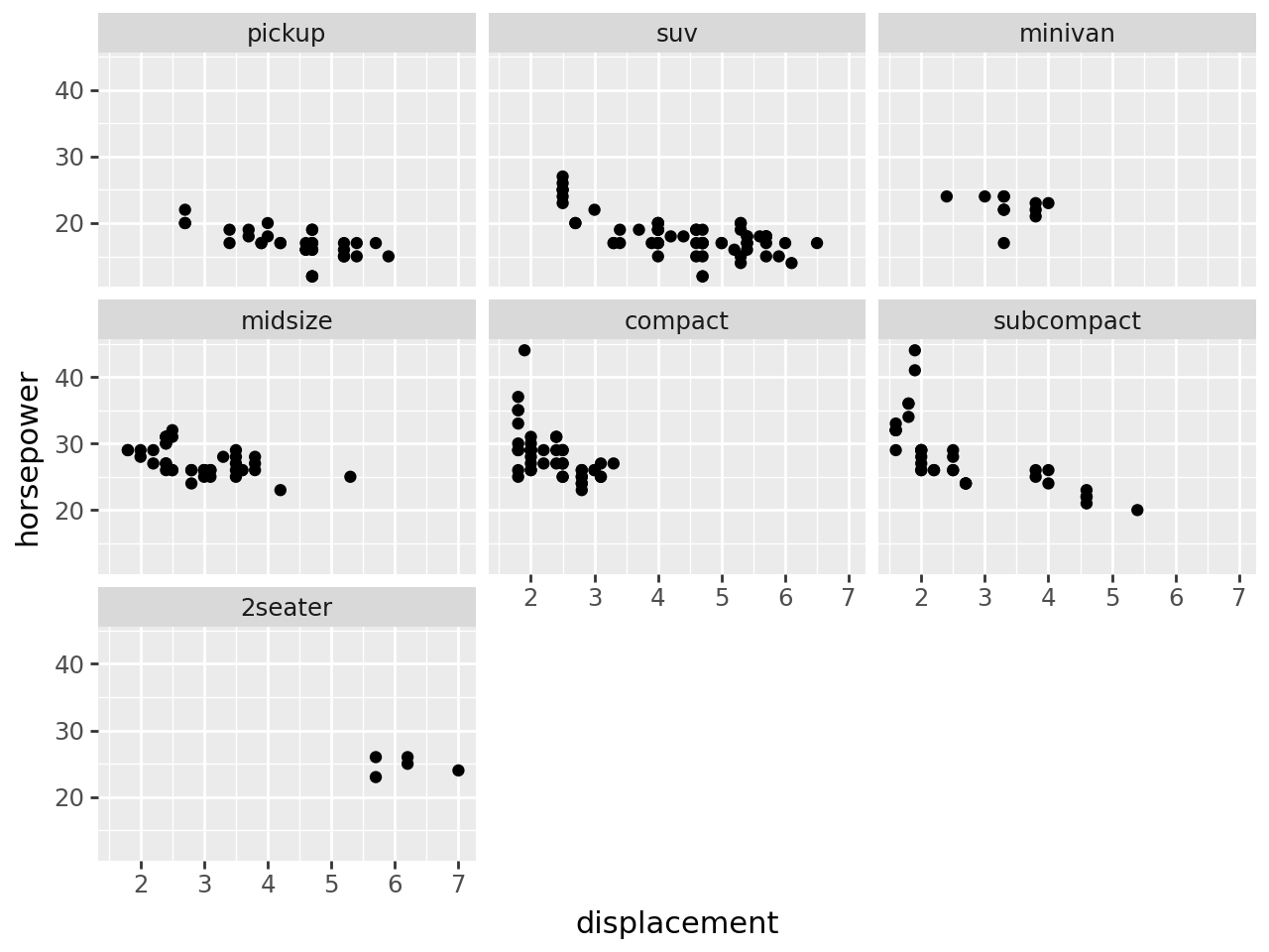
To change the plot order of the facets, use a categorical and reorder the levels of the faceting variable in the data.

mpg["class"] = mpg["class"].astype("category").cat.reorder_categories(
    ["pickup", "suv", "minivan", "midsize", "compact", "subcompact", "2seater"]
)

# facet plot with reorded drv category
(
    ggplot(mpg, aes(x="displ", y="hwy"))
    + geom_point()
    + facet_wrap("class")
    + labs(x="displacement", y="horsepower")
)

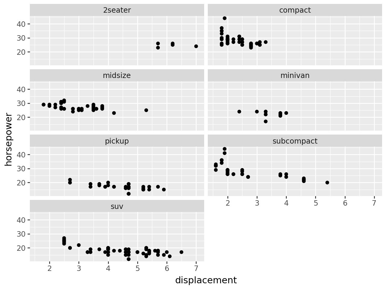
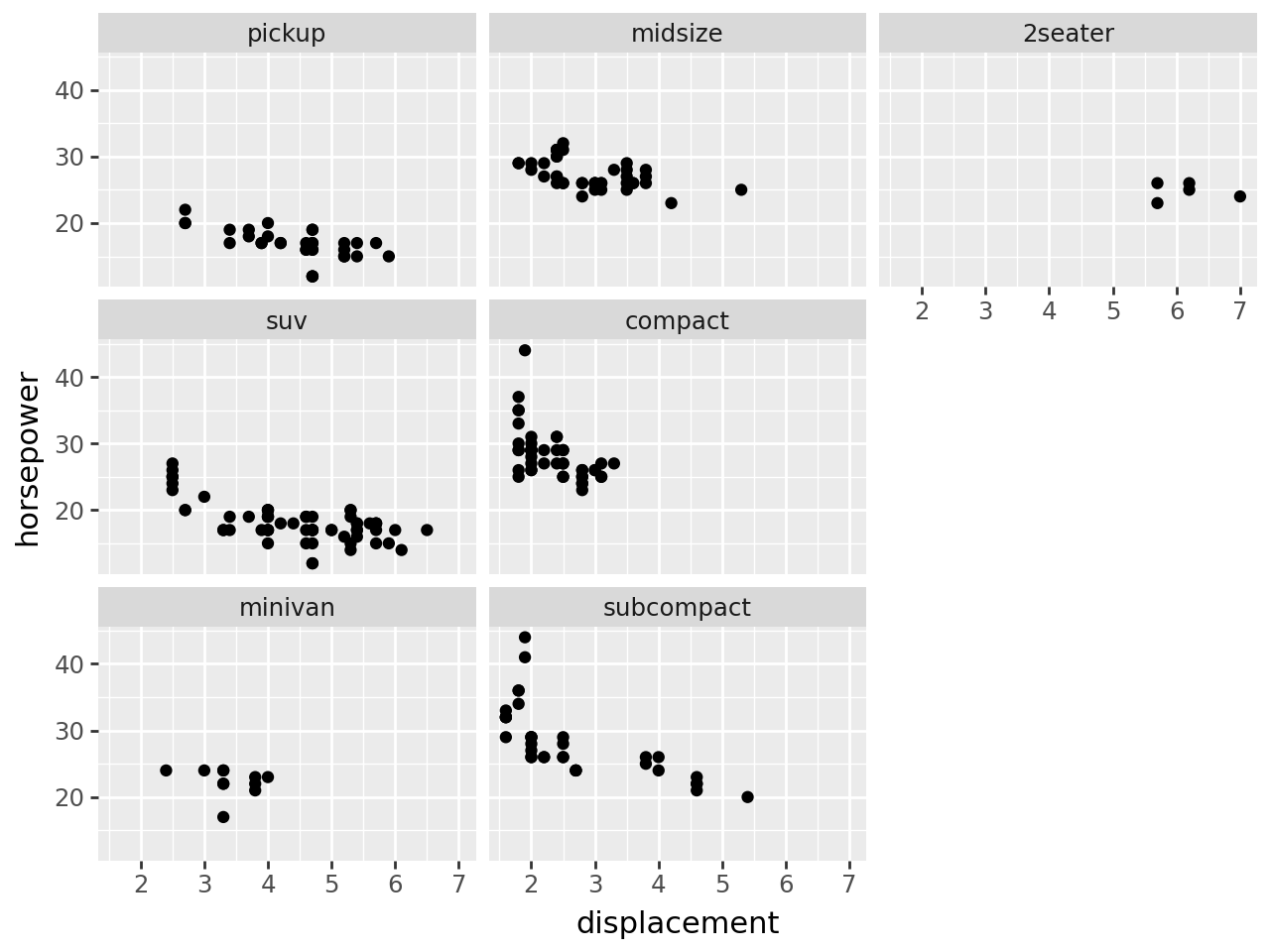
Ordinarily the facets are arranged horizontally (left-to-right from top to bottom). However if you would prefer a vertical layout (facets are arranged top-to-bottom, from left to right) use the dir option:

# Facet plot with vertical layout
(
    ggplot(mpg, aes(x="displ", y="hwy"))
    + geom_point()
    + facet_wrap(
        "class",
        dir="v",  # change to a vertical layout
    )
    + labs(x="displacement", y="horsepower")
)

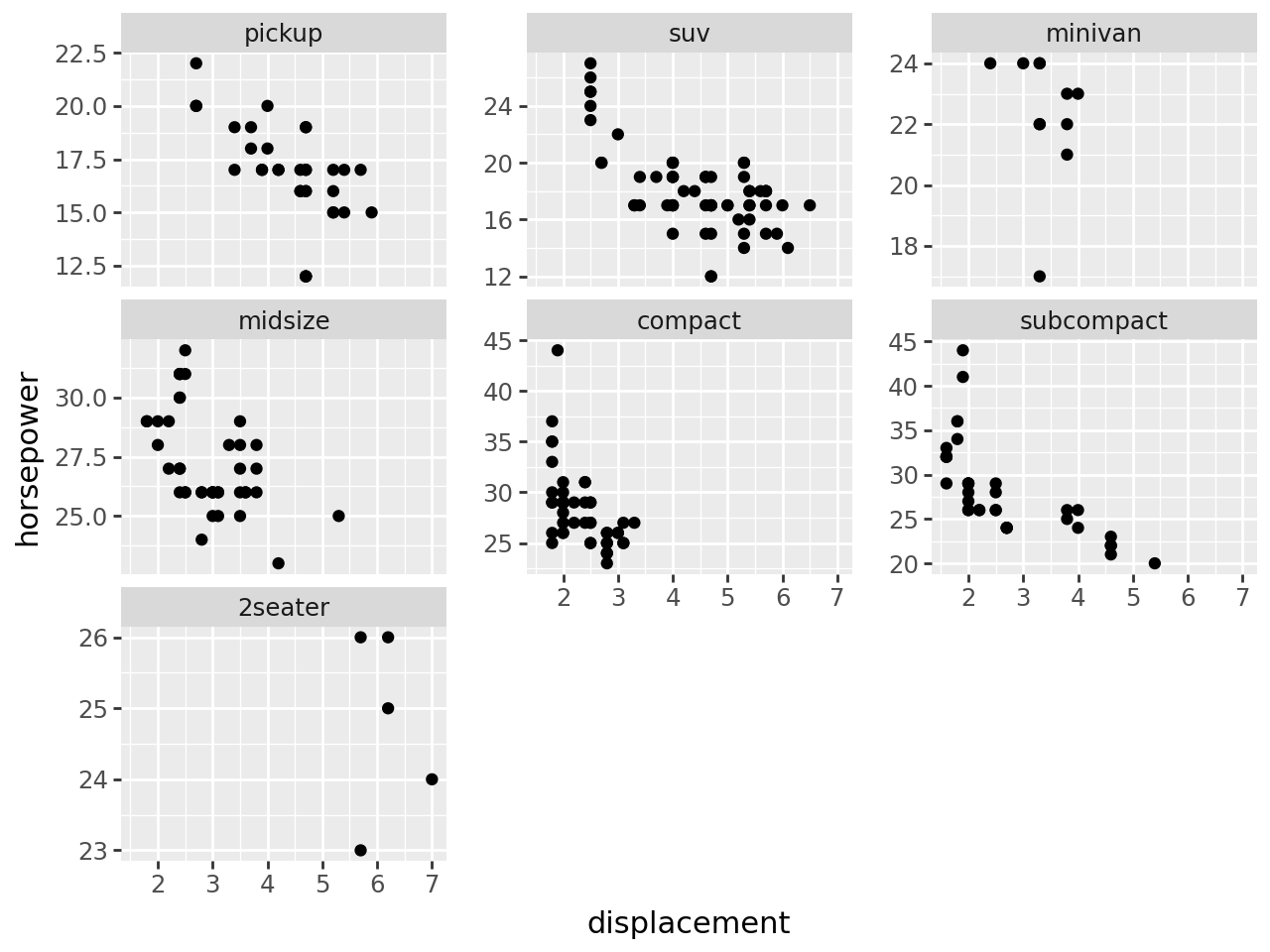
You can choose if the scale of x- and y-axes are fixed or variable. Set the scales argument to free-y, free_x or free for a free scales on the y-axis, x-axis or both axes respectively. You may need to add spacing between the facets to ensure axis ticks and values are easy to read.

A fixed scale is the default and does not need to be specified.

# facet plot with free scales
(
    ggplot(mpg, aes(x="displ", y="hwy"))
    + geom_point()
    + facet_wrap(
        "class",
        scales="free_y",  # set scales so y-scale varies with the data
    )
    + labs(x="displacement", y="horsepower")
)

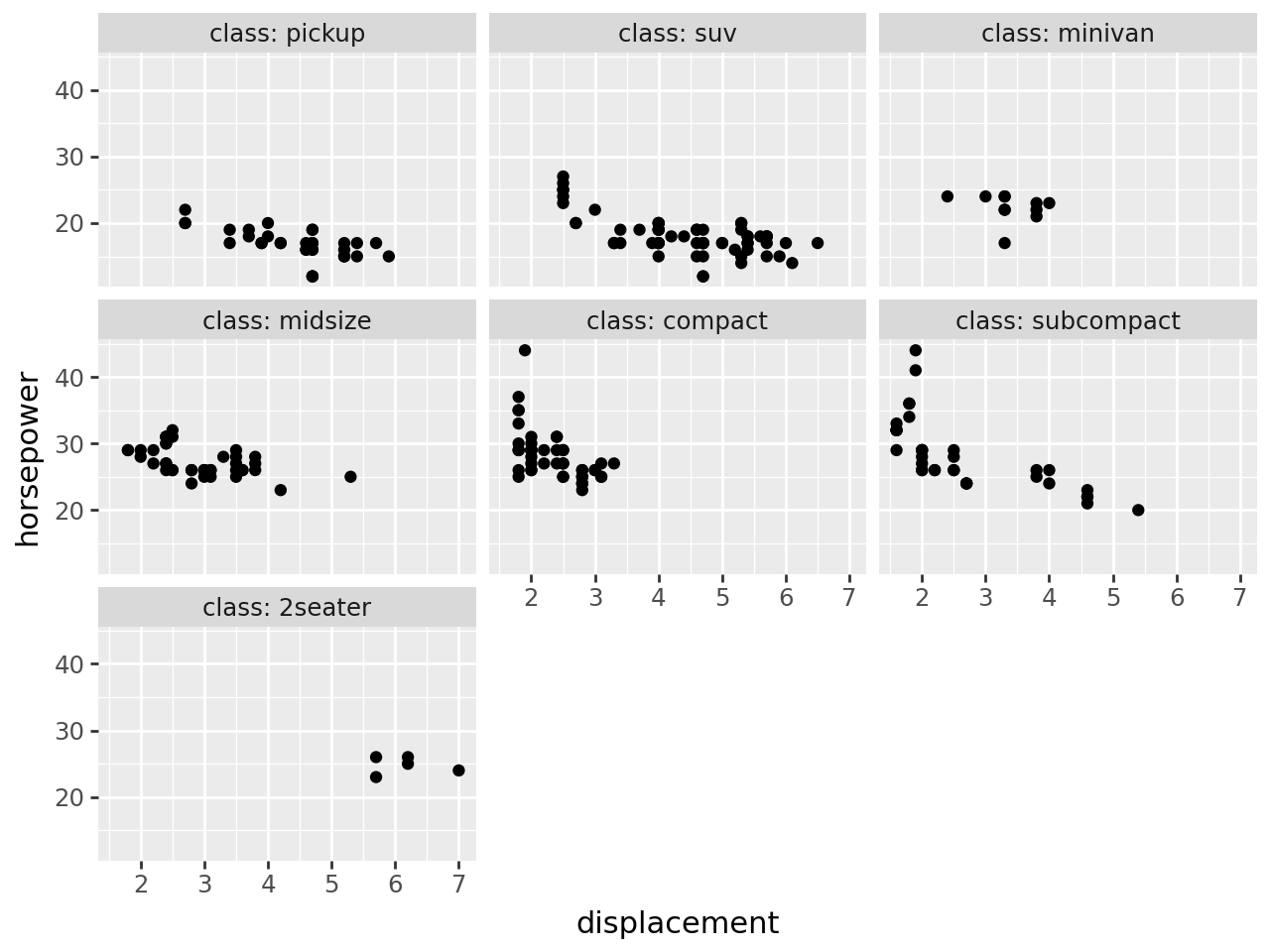
You can add additional information to your facet labels, by using the labeller argument within the facet_wrap() command. Below we use labeller = 'label_both' to include the column name in the facet label.

# facet plot with labeller
(
    ggplot(mpg, aes(x="displ", y="hwy"))
    + geom_point()
    + facet_wrap("class", labeller="label_both")
    + labs(x="displacement", y="horsepower")
)

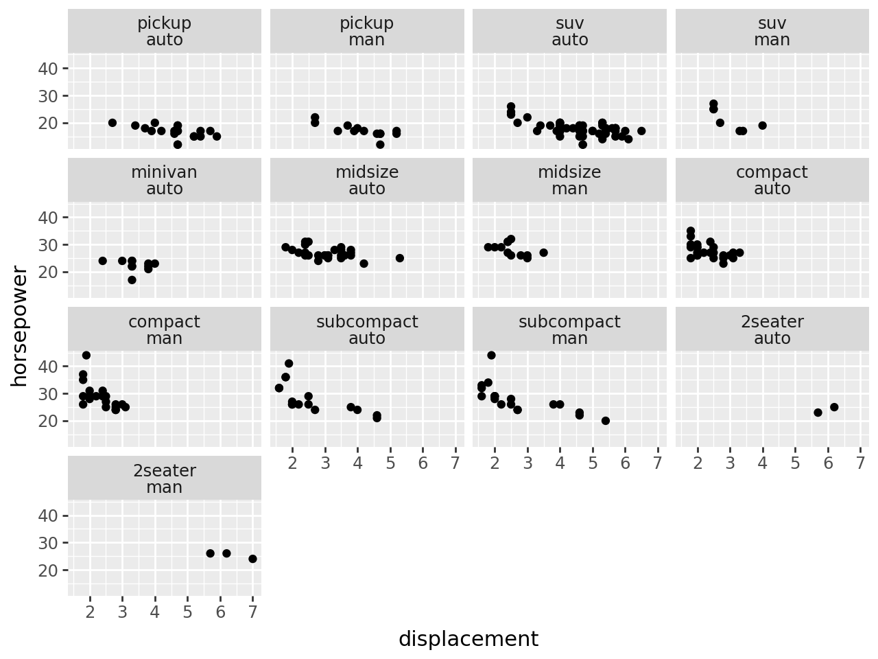
You can add two discrete variables to a facet:

# add additional column for plotting exercise
mpg["transmission"] = mpg["trans"].map(
    lambda x: "auto" if "auto" in x else "man" if "man" in x else ""
)

# inspect new column transmission which identifies cars as having an automatic or manual transmission
mpg.head()

	manufacturer	model	displ	year	cyl	trans	drv	cty	hwy	fl	class	transmission
0	audi	a4	1.8	1999	4	auto(l5)	f	18	29	p	compact	auto
1	audi	a4	1.8	1999	4	manual(m5)	f	21	29	p	compact	man
2	audi	a4	2.0	2008	4	manual(m6)	f	20	31	p	compact	man
3	audi	a4	2.0	2008	4	auto(av)	f	21	30	p	compact	auto
4	audi	a4	2.8	1999	6	auto(l5)	f	16	26	p	compact	auto

# facet plot with two variables on one facet
(
    ggplot(mpg, aes(x="displ", y="hwy"))
    + geom_point()
    + facet_wrap(["class", "transmission"])  # use a list to add additional facetting variables
    + labs(x="displacement", y="horsepower")
)