A box and whiskers plot

In [1]:

import numpy as np
import pandas as pd

from plotnine import (
    ggplot,
    aes,
    geom_boxplot,
    geom_jitter,
    scale_x_discrete,
    coord_flip,
)
from plotnine.data import pageviews

The boxplot compactly displays the distribution of a continuous variable.

Read more: + wikipedia + ggplot2 docs

In [2]:

flights = pd.read_csv("data/flights.csv")
flights.head()

	year	month	passengers
0	1949	January	112
1	1949	February	118
2	1949	March	132
3	1949	April	129
4	1949	May	121

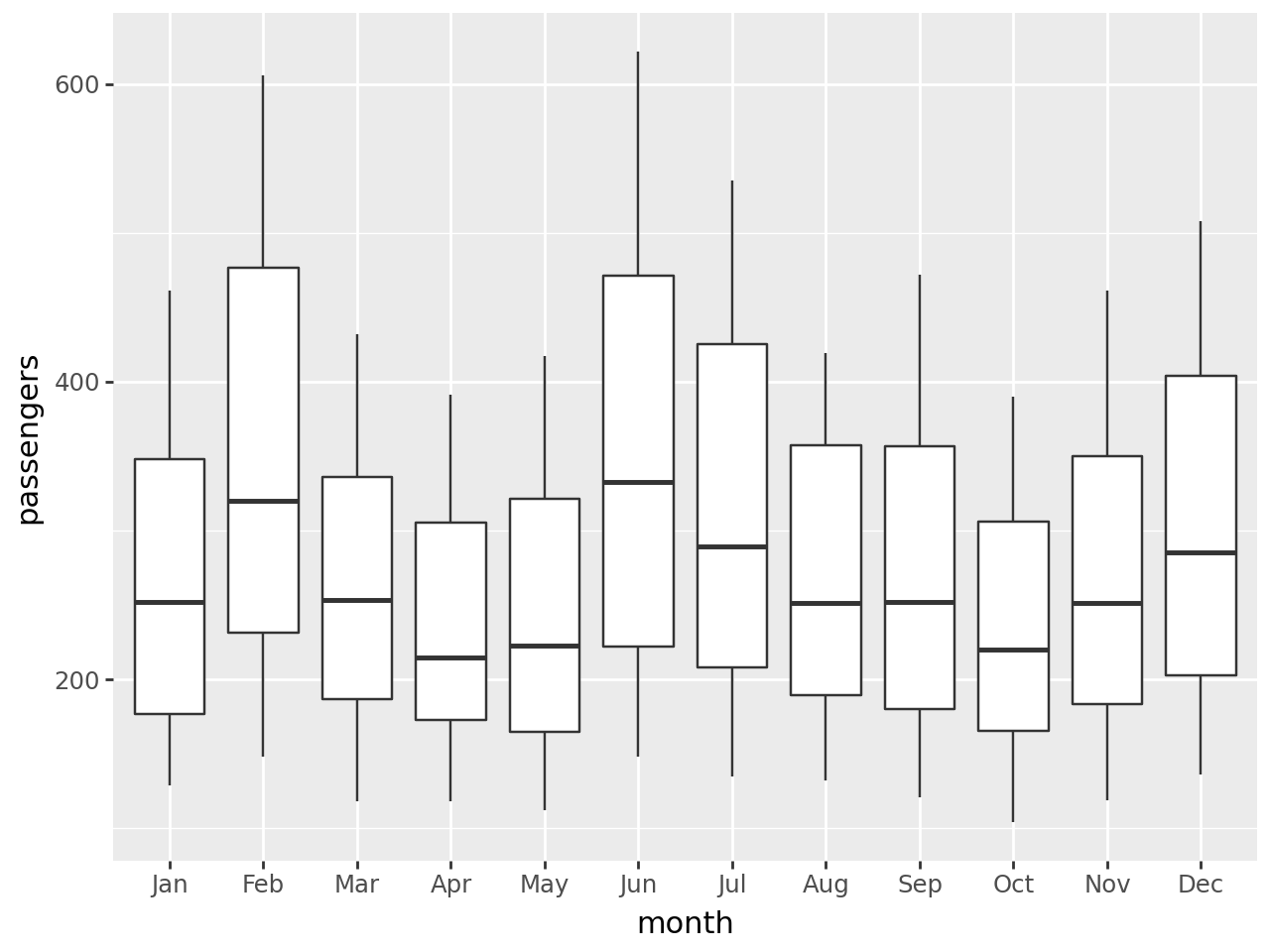
Basic boxplot

In [3]:

months = [month[:3] for month in flights.month[:12]]
print(months)

['Jan', 'Feb', 'Mar', 'Apr', 'May', 'Jun', 'Jul', 'Aug', 'Sep', 'Oct', 'Nov', 'Dec']

A Basic Boxplot

In [4]:

# Gallery, distributions
(
    ggplot(flights)
    + geom_boxplot(aes(x="factor(month)", y="passengers"))
    + scale_x_discrete(labels=months, name="month")  # change ticks labels on OX
)

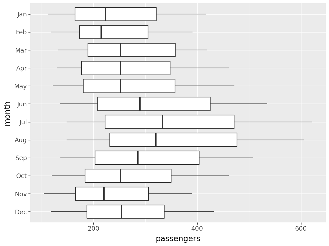
Horizontal boxplot

In [5]:

(
    ggplot(flights)
    + geom_boxplot(aes(x="factor(month)", y="passengers"))
    + coord_flip()
    + scale_x_discrete(
        labels=months[::-1],
        limits=flights.month[11::-1],
        name="month",
    )
)

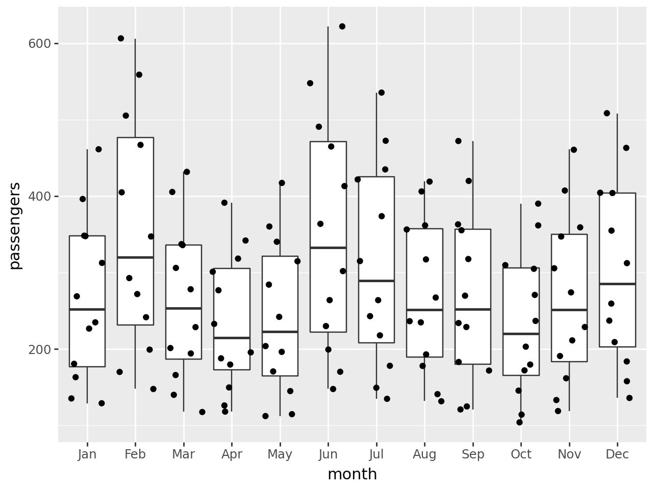
Boxplot with jittered points:

In [6]:

(
    ggplot(flights, aes(x="factor(month)", y="passengers"))
    + geom_boxplot()
    + geom_jitter()
    + scale_x_discrete(labels=months, name="month")  # change ticks labels on OX
)

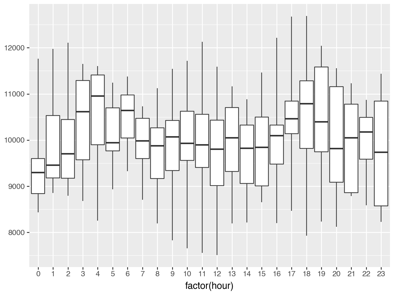
Precomputed boxplots

For datasets that do not fit in memory, you can precompute the boxplot metrics (for example by aggregating the statistics using database queries) and then use geom_boxplot with stat="identity".

In [7]:

# Precompute the metrics
def q25(x):
    return x.quantile(0.25)

def q75(x):
    return x.quantile(0.75)
    
pageviews["hour"] = pageviews.date_hour.dt.hour
precomputed_metrics = pageviews.groupby("hour").agg({'pageviews': ["min", q25, "median", q75, "max"]})
precomputed_metrics.columns = [col_name[1] for col_name in precomputed_metrics.columns]  
precomputed_metrics = precomputed_metrics.reset_index()
precomputed_metrics.head()

	hour	min	q25	median	q75	max
0	0	8437.500380	8842.109077	9297.046035	9600.362430	11762.446233
1	1	8852.123978	9177.938537	9457.821814	10530.072887	11974.437292
2	2	8793.076686	9176.462389	9704.885172	10446.315276	12105.406628
3	3	8683.606449	9574.722286	10615.670464	11290.246605	11651.443193
4	4	8252.974951	9898.998785	10959.909095	11409.657288	11603.711837

In [8]:

(
    ggplot(precomputed_metrics)
    + geom_boxplot(
        aes(x="factor(hour)", ymin="min", lower="q25", middle="median", upper="q75", ymax="max"),
        stat="identity"
    )
)