plotnine.facet_wrap

facet_wrap(
    facets=None,
    *,
    nrow=None,
    ncol=None,
    scales="fixed",
    shrink=True,
    labeller="label_value",
    as_table=True,
    drop=True,
    dir="h"
)

Wrap 1D Panels onto 2D surface

Parameters

facets : Optional[str | Sequence[str]] = None

Variables to groupby and plot on different panels. If a string formula is used it should be right sided, e.g "~ a + b", ("a", "b")

nrow : int = None

Number of rows

ncol : int = None

Number of columns

scales : Literal["fixed", "free", "free_x", "free_y"] = "fixed"

Whether x or y scales should be allowed (free) to vary according to the data on each of the panel.

shrink : bool = True

Whether to shrink the scales to the output of the statistics instead of the raw data.

labeller : Literal["label_value", "label_both", "label_context"] = "label_value"

How to label the facets. A string value if it should be one of ["label_value", "label_both", "label_context"].

as_table : bool = True

If True, the facets are laid out like a table with the highest values at the bottom-right. If False the facets are laid out like a plot with the highest value a the top-right

drop : bool = True

If True, all factor levels not used in the data will automatically be dropped. If False, all factor levels will be shown, regardless of whether or not they appear in the data.

dir : Literal["h", "v"] = "h"

Direction in which to layout the panels. h for horizontal and v for vertical.

Examples

from plotnine import ggplot, aes, geom_point, labs, facet_wrap, theme
from plotnine.data import mpg

Facet wrap

facet_wrap() creates a collection of plots (facets), where each plot is differentiated by the faceting variable. These plots are wrapped into a certain number of columns or rows as specified by the user.

mpg.head()

	manufacturer	model	displ	year	cyl	trans	drv	cty	hwy	fl	class
0	audi	a4	1.8	1999	4	auto(l5)	f	18	29	p	compact
1	audi	a4	1.8	1999	4	manual(m5)	f	21	29	p	compact
2	audi	a4	2.0	2008	4	manual(m6)	f	20	31	p	compact
3	audi	a4	2.0	2008	4	auto(av)	f	21	30	p	compact
4	audi	a4	2.8	1999	6	auto(l5)	f	16	26	p	compact

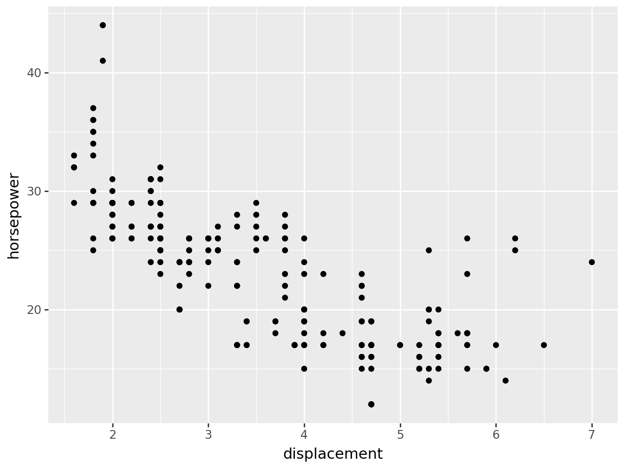
Basic scatter plot:

(
    ggplot(mpg, aes(x="displ", y="hwy"))
    + geom_point()
    + labs(x="displacement", y="horsepower")
)

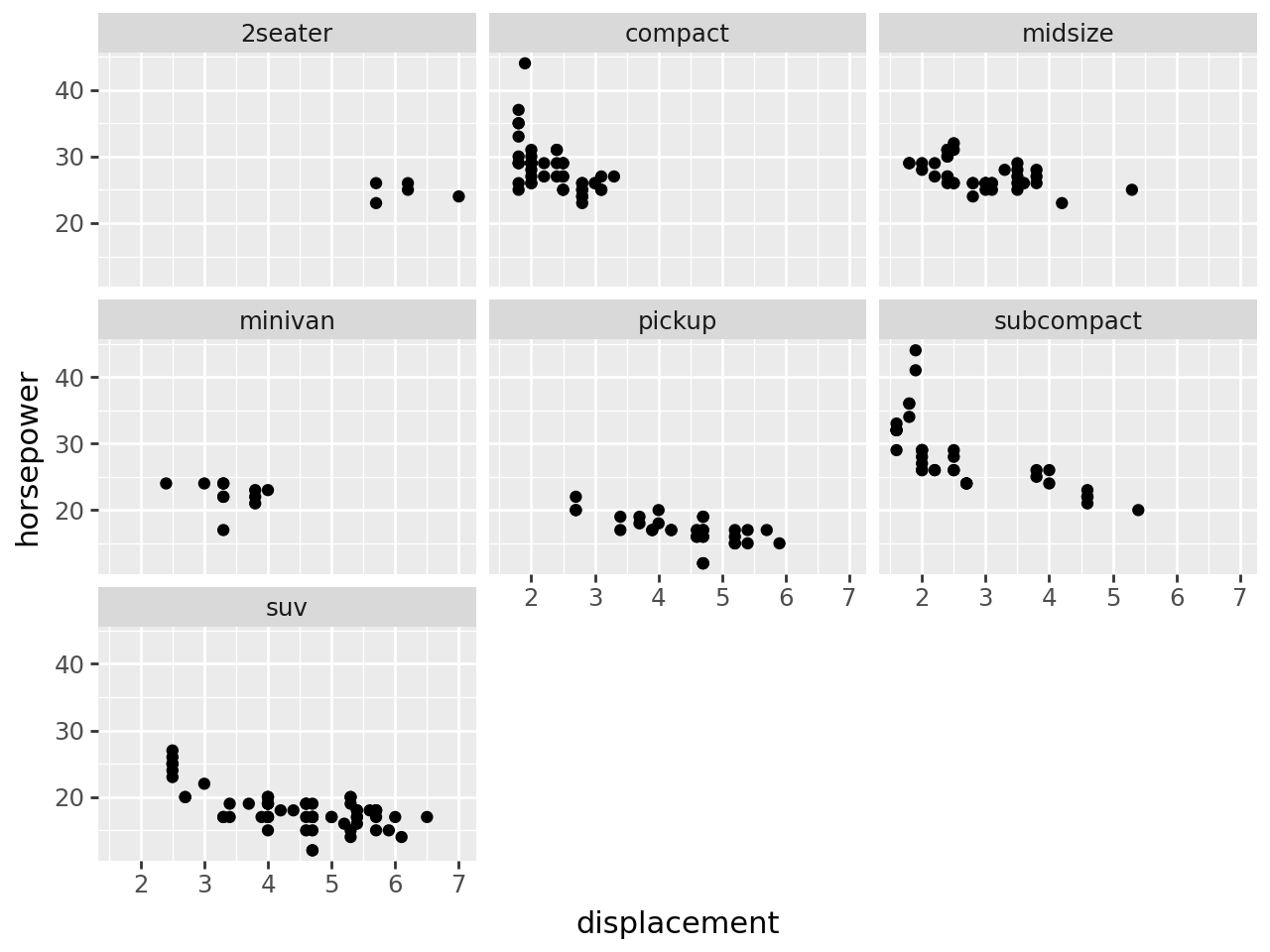
Facet a discrete variable using facet_wrap():

(
    ggplot(mpg, aes(x="displ", y="hwy"))
    + geom_point()
    + facet_wrap("class")
    + labs(x="displacement", y="horsepower")
)

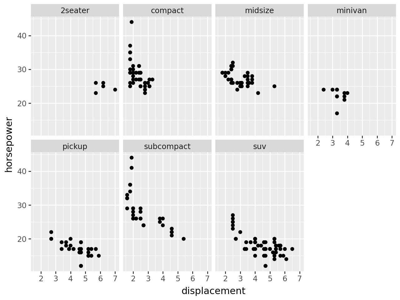
Control the number of rows and columns with the options nrow and ncol:

# Selecting the number of columns to display
(
    ggplot(mpg, aes(x="displ", y="hwy"))
    + geom_point()
    + facet_wrap(
        "class",
        ncol=4,  # change the number of columns
    )
    + labs(x="displacement", y="horsepower")
)

# Selecting the number of rows to display

(
    ggplot(mpg, aes(x="displ", y="hwy"))
    + geom_point()
    + facet_wrap(
        "class",
        nrow=4,  # change the number of columns
    )
    + labs(x="displacement", y="horsepower")
)

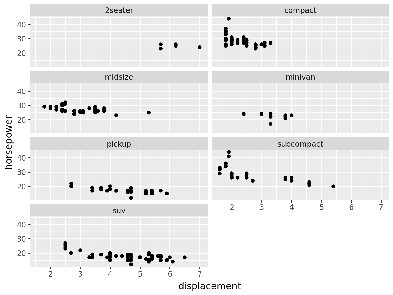
To change the plot order of the facets, reorder the levels of the faceting variable in the data.

# re-order categories
mpg["class"] = mpg["class"].cat.reorder_categories(
    ["pickup", "suv", "minivan", "midsize", "compact", "subcompact", "2seater"]
)

# facet plot with reorded drv category
(
    ggplot(mpg, aes(x="displ", y="hwy"))
    + geom_point()
    + facet_wrap("class")
    + labs(x="displacement", y="horsepower")
)

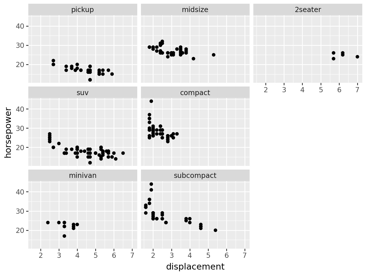
Ordinarily the facets are arranged horizontally (left-to-right from top to bottom). However if you would prefer a vertical layout (facets are arranged top-to-bottom, from left to right) use the dir option:

# Facet plot with vertical layout
(
    ggplot(mpg, aes(x="displ", y="hwy"))
    + geom_point()
    + facet_wrap(
        "class",
        dir="v",  # change to a vertical layout
    )
    + labs(x="displacement", y="horsepower")
)

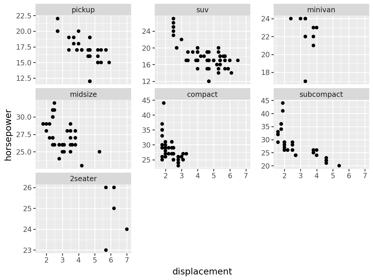
You can choose if the scale of x- and y-axes are fixed or variable. Set the scales argument to free-y, free_x or free for a free scales on the y-axis, x-axis or both axes respectively. You may need to add spacing between the facets to ensure axis ticks and values are easy to read.

A fixed scale is the default and does not need to be specified.

# facet plot with free scales
(
    ggplot(mpg, aes(x="displ", y="hwy"))
    + geom_point()
    + facet_wrap(
        "class",
        scales="free_y",  # set scales so y-scale varies with the data
    )
    + labs(x="displacement", y="horsepower")
)

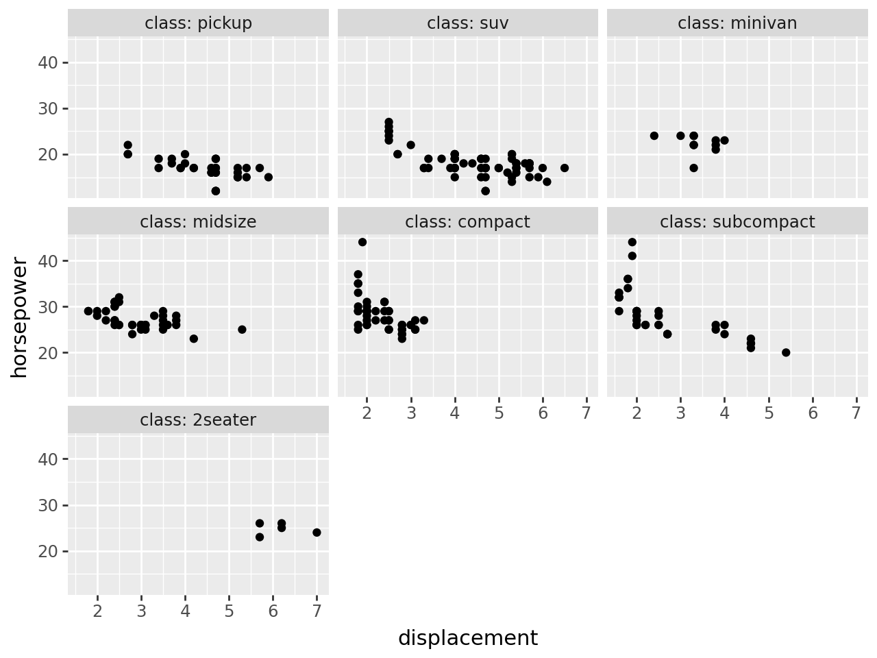
You can add additional information to your facet labels, by using the labeller argument within the facet_wrap() command. Below we use labeller = 'label_both' to include the column name in the facet label.

# facet plot with labeller
(
    ggplot(mpg, aes(x="displ", y="hwy"))
    + geom_point()
    + facet_wrap("class", labeller="label_both")
    + labs(x="displacement", y="horsepower")
)

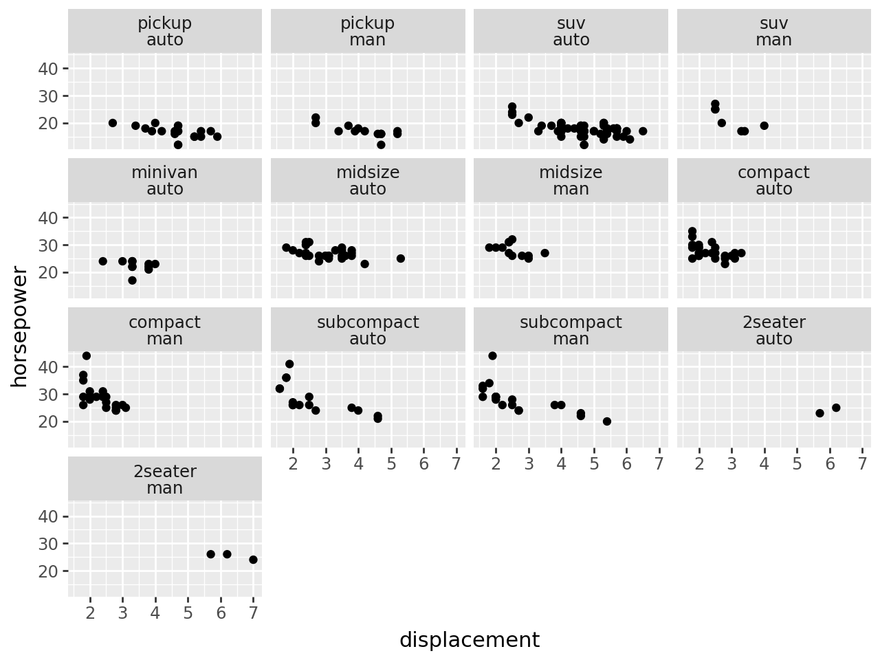
You can add two discrete variables to a facet:

# add additional column for plotting exercise
mpg["transmission"] = mpg["trans"].map(
    lambda x: "auto" if "auto" in x else "man" if "man" in x else ""
)

# inspect new column transmission which identifies cars as having an automatic or manual transmission
mpg.head()

	manufacturer	model	displ	year	cyl	trans	drv	cty	hwy	fl	class	transmission
0	audi	a4	1.8	1999	4	auto(l5)	f	18	29	p	compact	auto
1	audi	a4	1.8	1999	4	manual(m5)	f	21	29	p	compact	man
2	audi	a4	2.0	2008	4	manual(m6)	f	20	31	p	compact	man
3	audi	a4	2.0	2008	4	auto(av)	f	21	30	p	compact	auto
4	audi	a4	2.8	1999	6	auto(l5)	f	16	26	p	compact	auto

# facet plot with two variables on one facet
(
    ggplot(mpg, aes(x="displ", y="hwy"))
    + geom_point()
    + facet_wrap(["class", "transmission"])  # use a list to add additional facetting variables
    + labs(x="displacement", y="horsepower")
)

Source: Facet wrap