from plotnine import (
    ggplot,
    aes,
    geom_point,
    geom_boxplot,
    geom_bar,
    geom_smooth,
    facet_wrap,
    labs,
    theme,
    theme_538,
    element_rect,
    element_text,
)
from plotnine import *
from plotnine.composition import plot_spacer
from plotnine.data import mtcars
Compose(items)Base class for those that create plot compositions
As a user, you will never directly work with this class, except through the operators that it makes possible. The operators are of two kinds:
1. Composing Operators
The combine plots or compositions into a single composition. Both operands are either a plot or a composition.
2. Plot Modifying Operators
The modify all or some of the plots in a composition. The left operand is a composition and the right operand is a plotaddable; any object that can be added to a ggplot object e.g. geoms, stats, themes, facets, … .
&-
Add right hand side to all plots in the composition.
*-
Add right hand side to all plots in the top-most nesting level of the composition.
+-
Add right hand side to the last plot in the composition.
Parameter Attributes
See Also
Beside-
To arrange plots side by side
Stack-
To arrange plots vertically
plot_spacer-
To add a blank space between plots
Examples
Plots
p1 = ggplot(mtcars, aes("disp", "qsec")) + geom_smooth()
p2 = ggplot(mtcars, aes("wt", "mpg")) + geom_point()
p3 = ggplot(mtcars, aes("factor(gear)", "mpg")) + geom_boxplot()
p4 = ggplot(mtcars, aes("carb")) + geom_bar()
The Arithmetic
(p1 | p2 | p3) / p4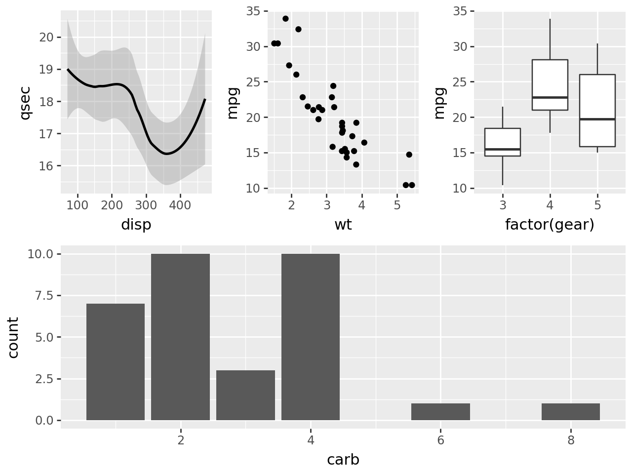
(p1 / p2 / p3) | p4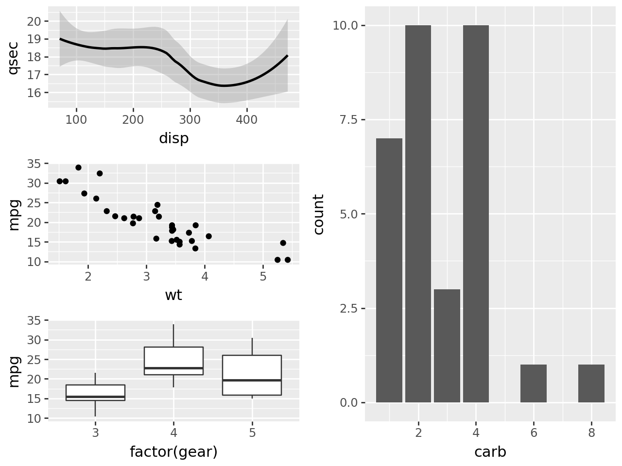
The grouping of the plots is determined by the precedence of the operators which means these two:
p1 / p2 / p3 | p4
(p1 / p2 / p3) | p4
are equivalent.
The space allocated within the overall composition is determined by the groups. e.g. Below, the panel in p1 has the same height as the panels of p2 and p3 combined.
(p1 / (p2 / p3)) | p4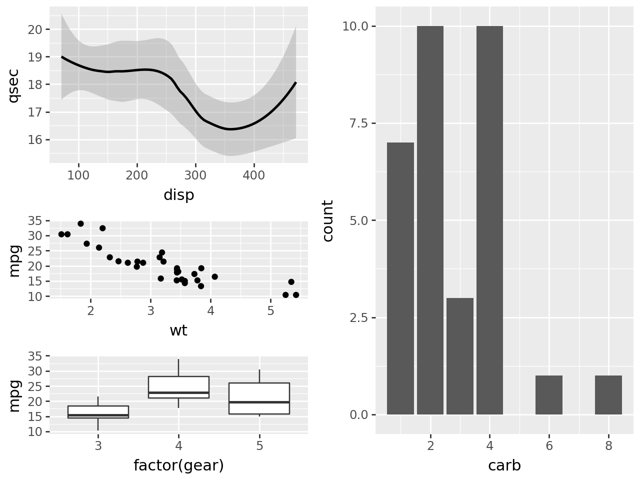
p1 | (p2 / p3) | p4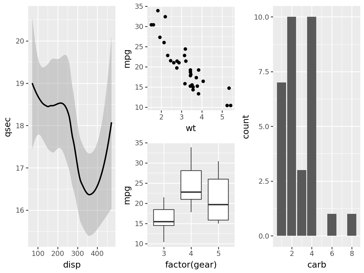
For a 2x wider panel on the left, we group the items on the right.
p1 | ((p2 / p3) | p4)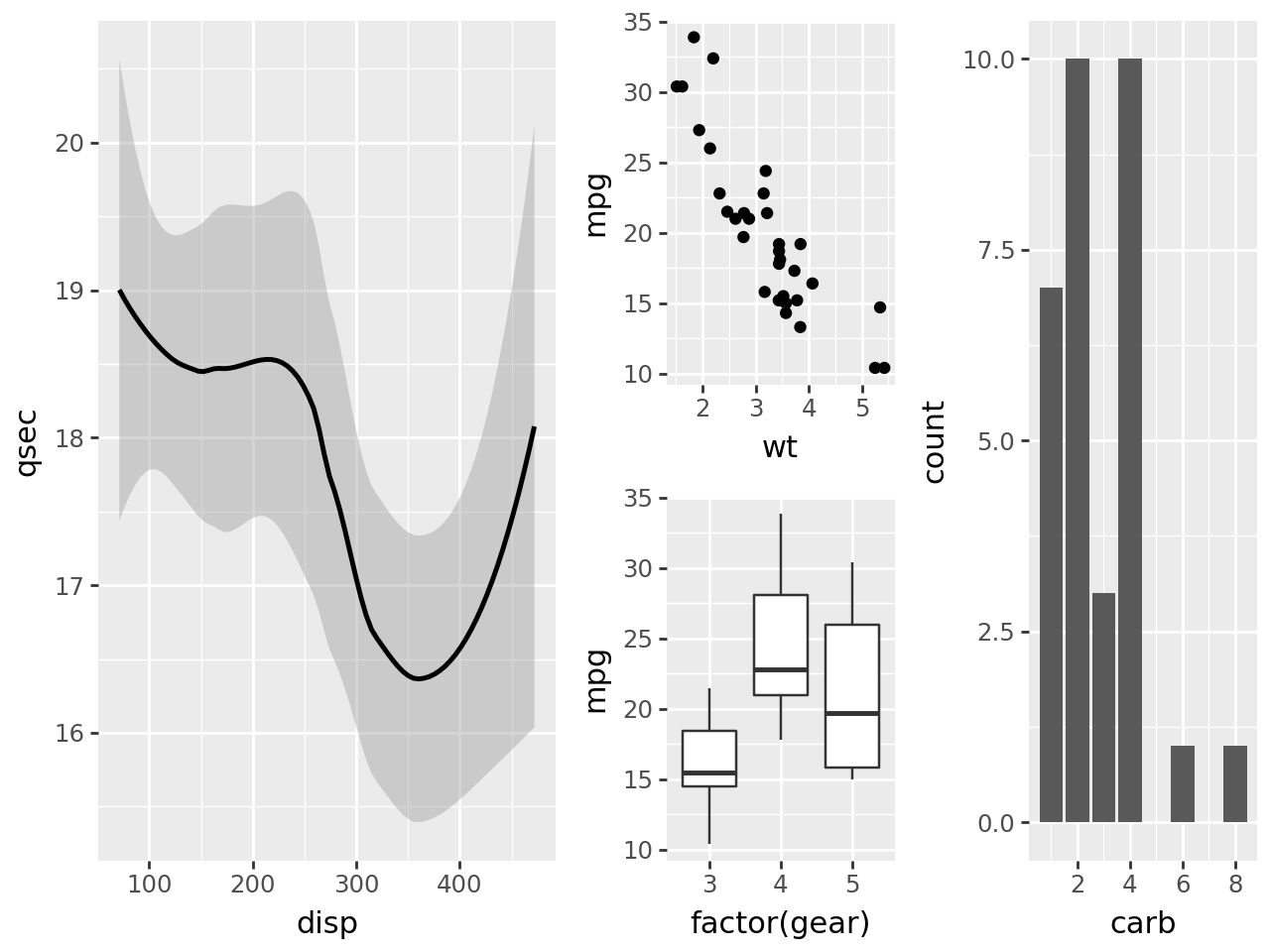
For a 2x wider panel on the right, we put together the left and right at the same nesting level.
(p1 | (p2 / p3)) - p4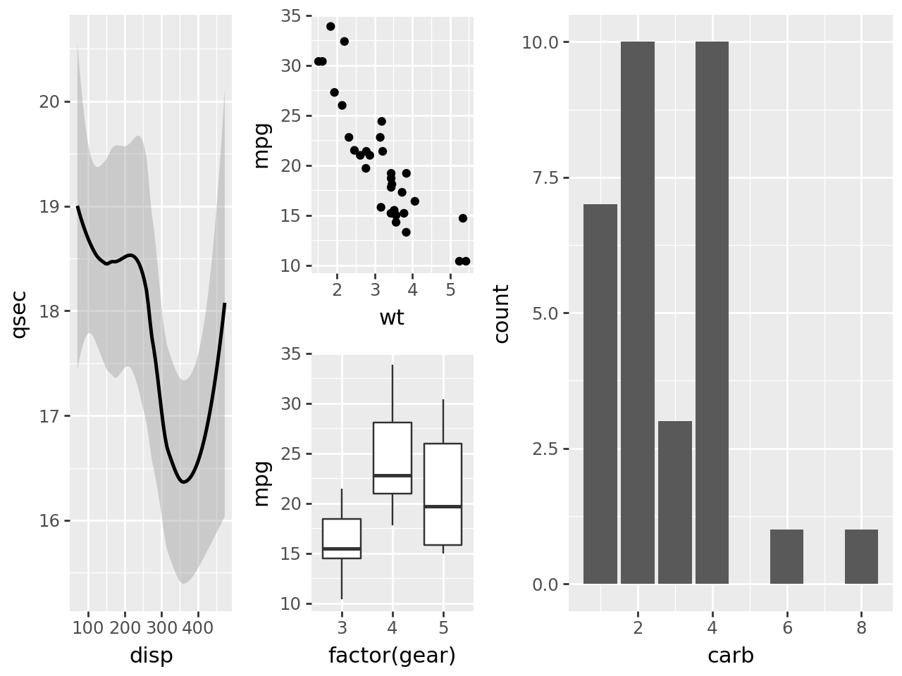
Modifying the composition
Add to the last plot in the composition
When an object that is not a plot or composition is added (+) to the composition, it is added (+) to the last plot in the composition.
composition = (p1 | (p2 / p3) | p4)
composition + theme_bw()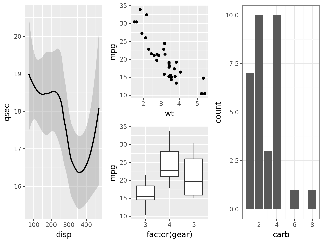
The dpi and figure_size of the composition are taken from the last plot, so we can add to the composition to change them.
composition + theme(figure_size=(4, 3))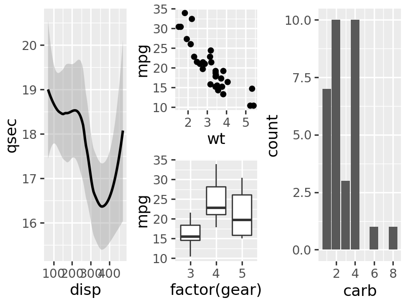
composition + geom_line(aes(y=after_stat("count")), stat="count", color="cyan")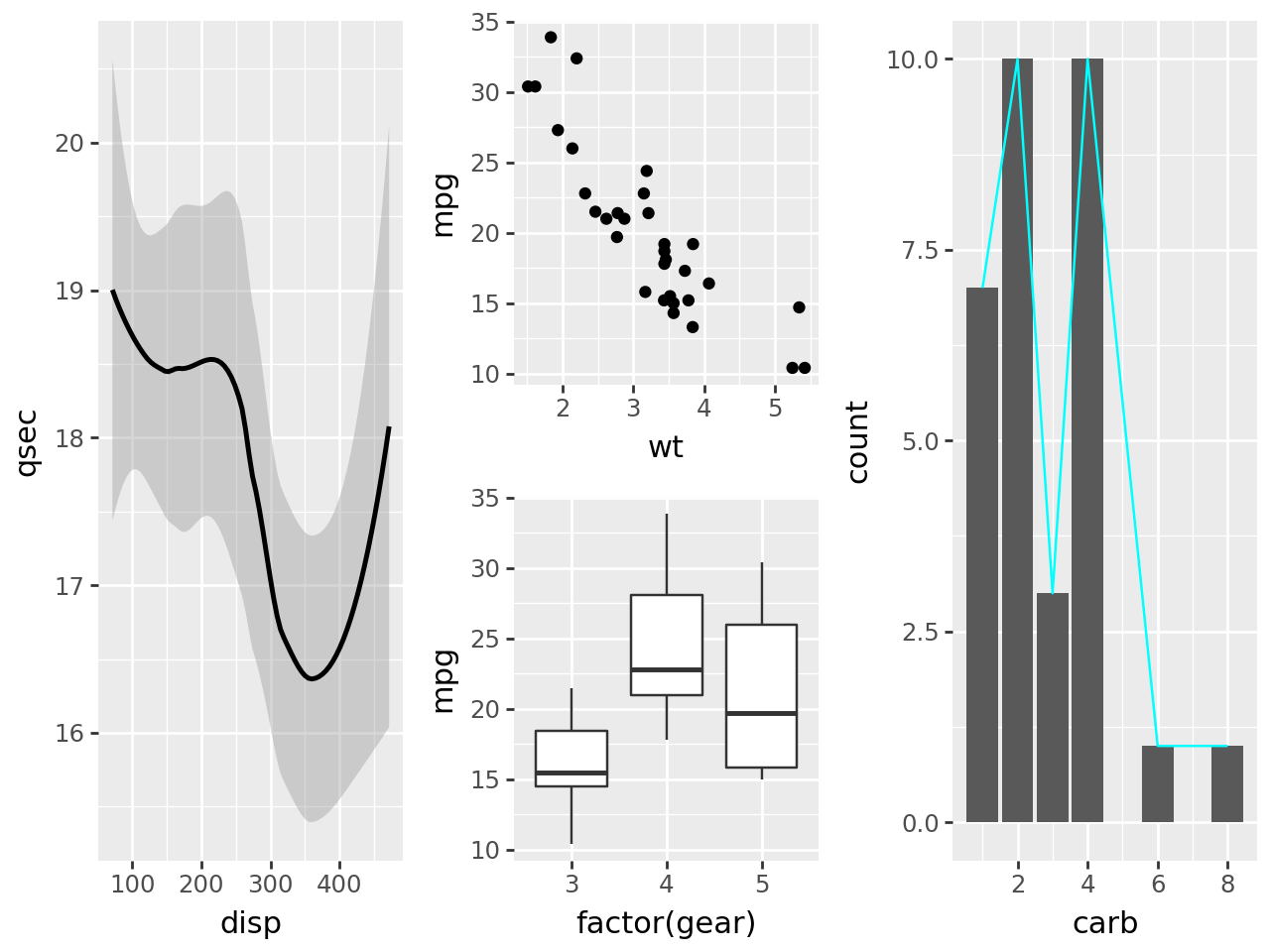
Add to plots at the top level of the composition
composition * theme_bw()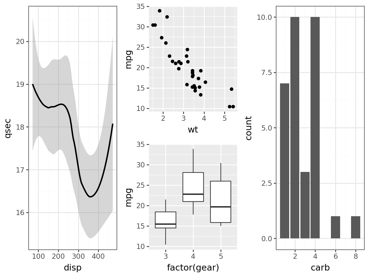
Add to all plots in the composition
composition & theme_bw()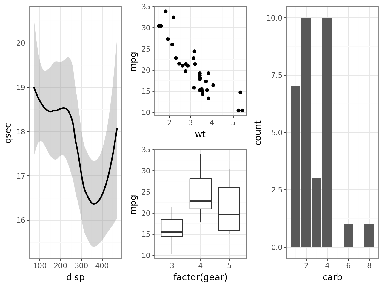
Adding space to the composition
You can create space within the composition by adding a plot_spacer or by adjusting plot_margin.
p1 | p2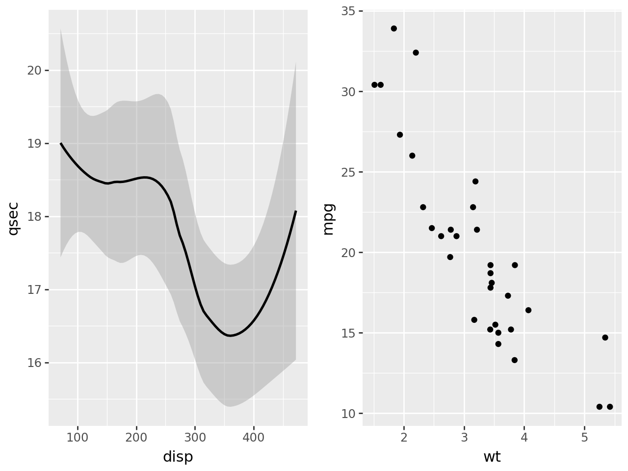
p1 | plot_spacer() | p2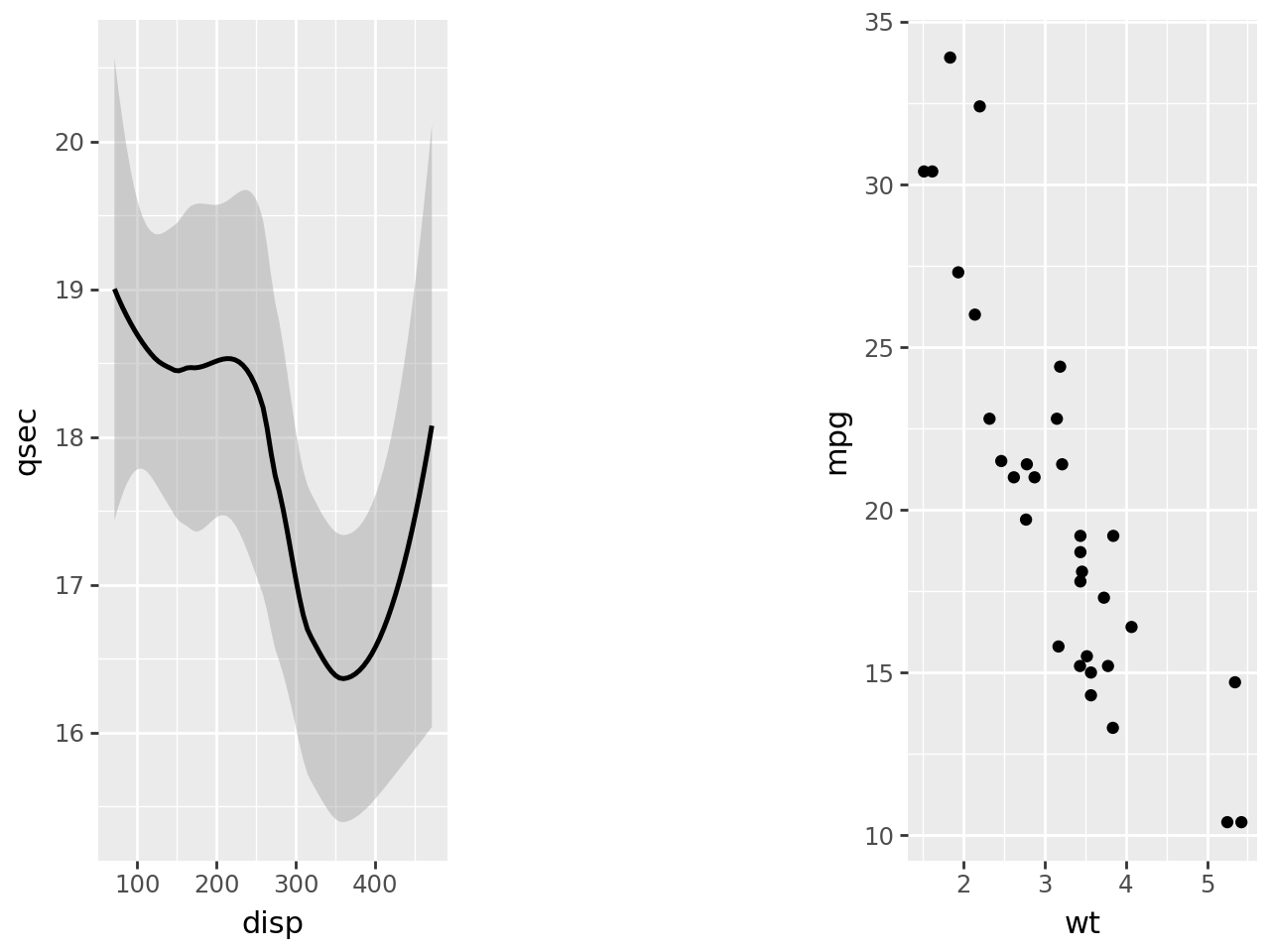
p1 | (p2 + theme(plot_margin_left=.25))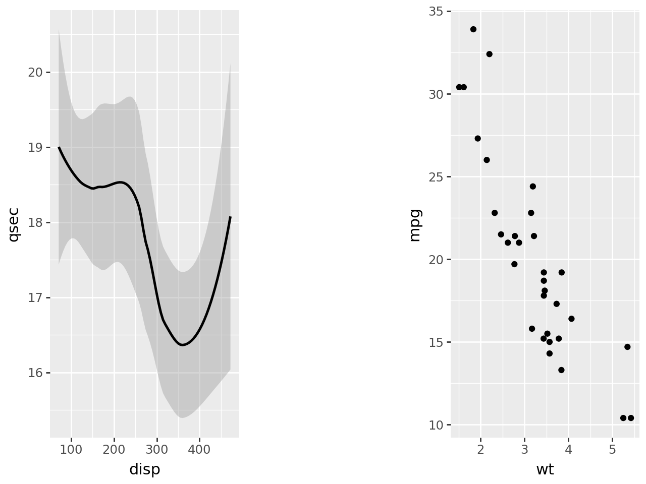
p1 | (p2 + theme(plot_margin_right=.25))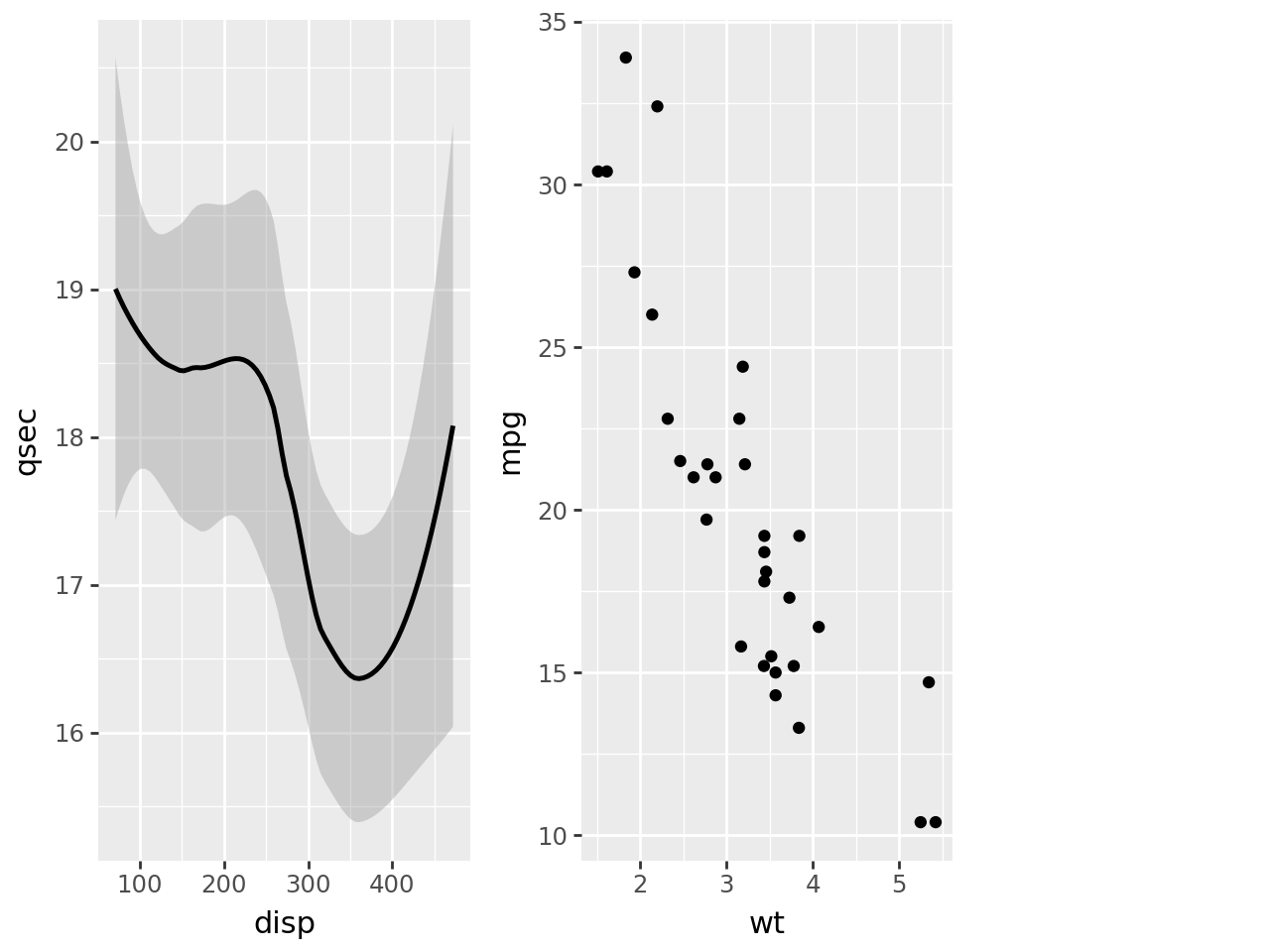
p1 | (p2 + theme(plot_margin_bottom=.25))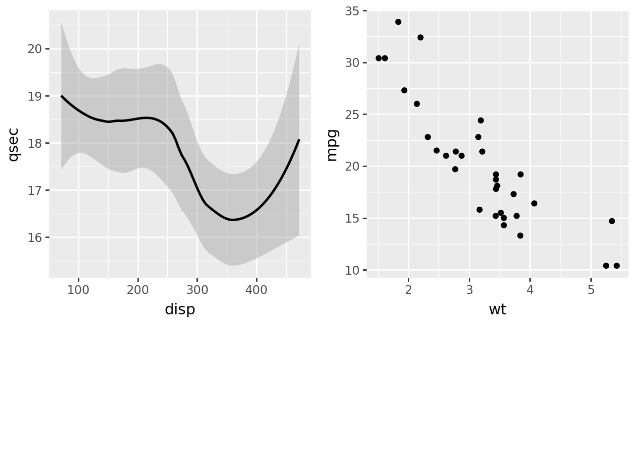
While the margin is added to p2, the height of p1 is adjusted so that the panels align.
How space is allocated
For any composition group, the space is allocated such that the edges of the panels align along one dimension, and the sizes are equal along the other dimension. For example, when a plot has a legend, it is allocated more space so that its panel has the same size as the adjacent panel.
p1 | p2 + aes(color="factor(cyl)")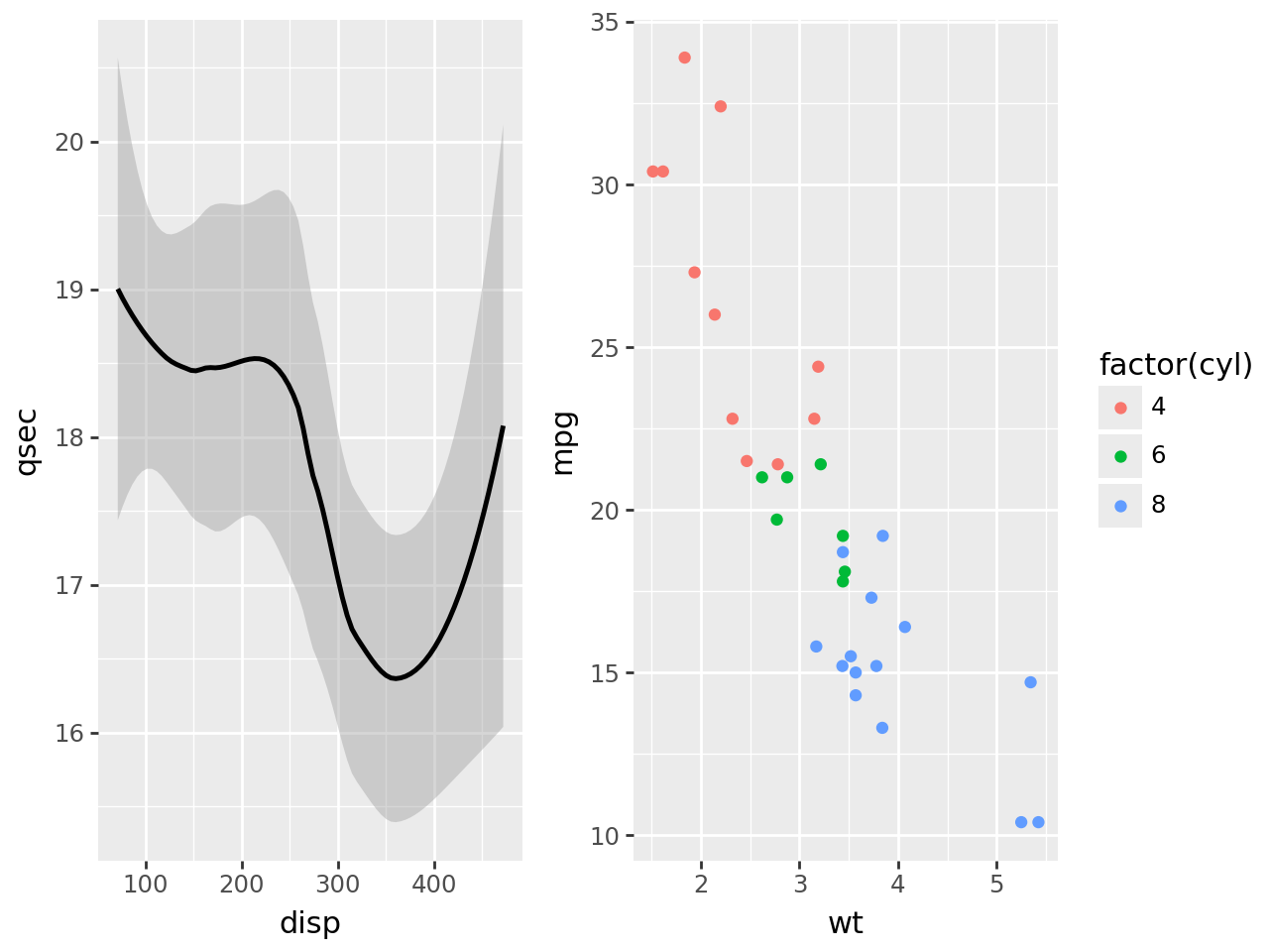
Making the plot backgrounds visible reveals the size of each plot.
brown_bg = theme(plot_background=element_rect(fill="#FF000022"))
cyan_bg = theme(plot_background=element_rect(fill="#00FF0022"))

(p1 + brown_bg) | (p2 + aes(color="factor(cyl)") + cyan_bg)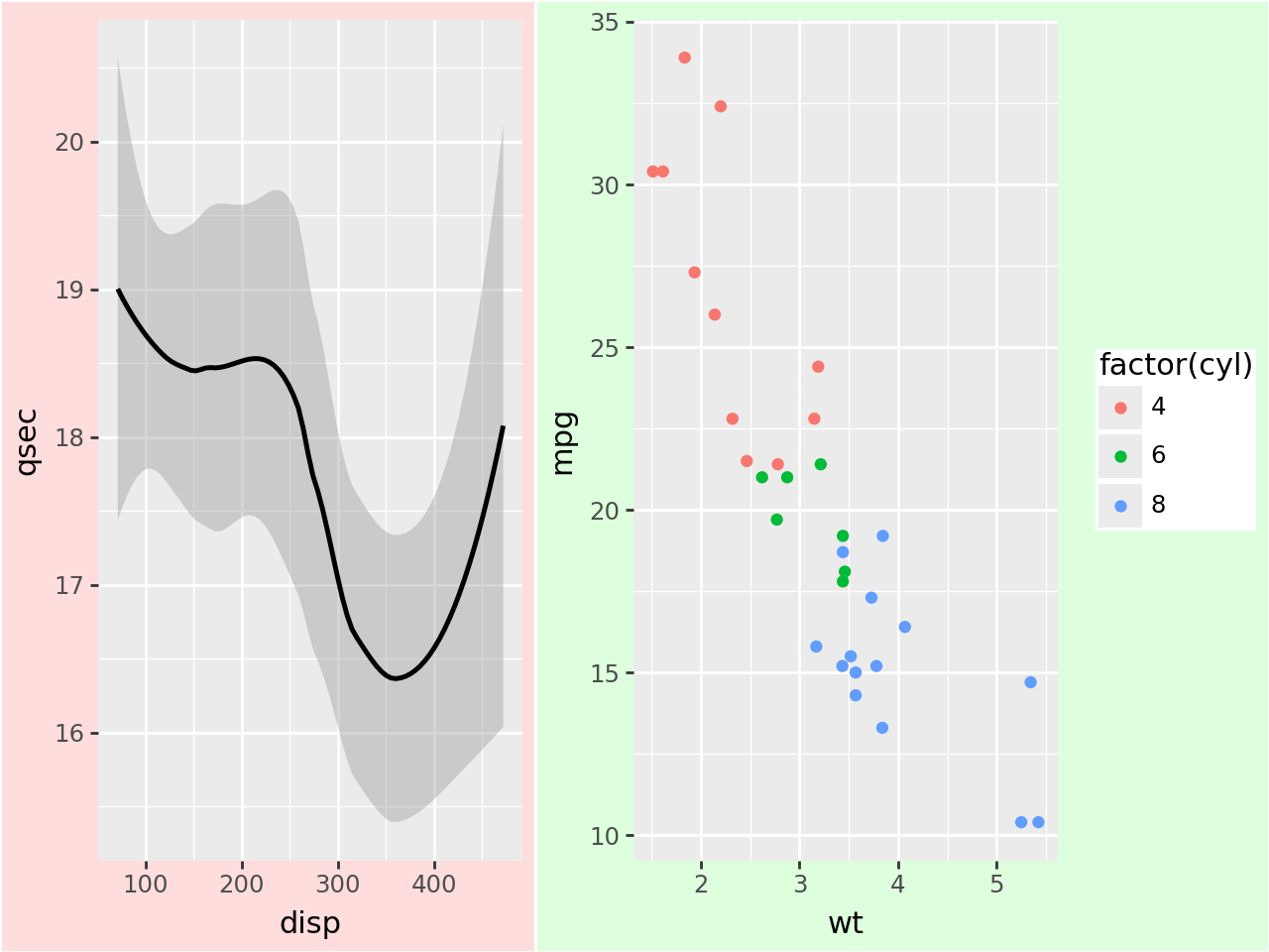
Facetted plots are treated as if all the panels were one.
p1 | (p2 + aes(color="factor(cyl)") + facet_wrap("cyl", ncol=1))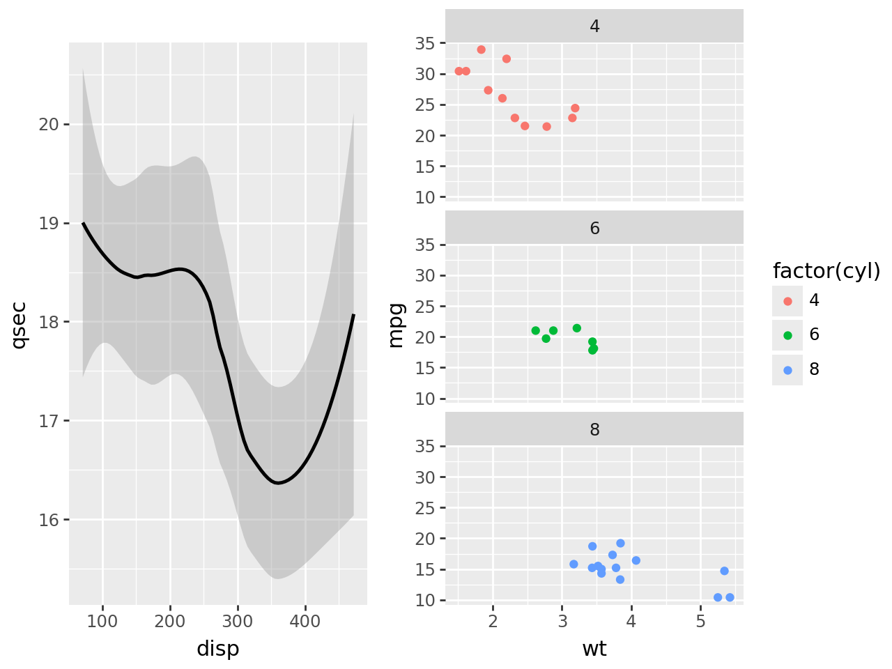
And the space between the facet panels counts towards the panel area of the plot.
p1 | (p2 + aes(color="factor(cyl)") + facet_wrap("cyl", ncol=2))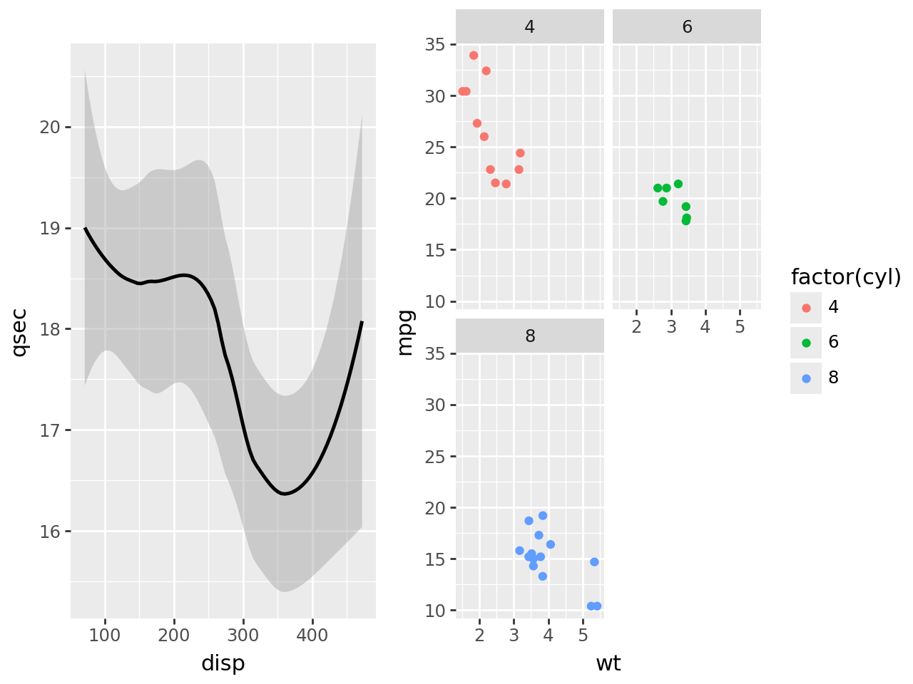
Tagging Plots
Tags are an essential part of plot compositions and the by default the are placed in the top-left margin of each plot.
p1_a = p1 + labs(tag="a)")
p2_b = p2 + labs(tag="b)")
p3_c = p3 + labs(tag="c)")
p4_d = p4 + labs(tag="d)")

(p1_a | p2_b | p3_c) / p4_d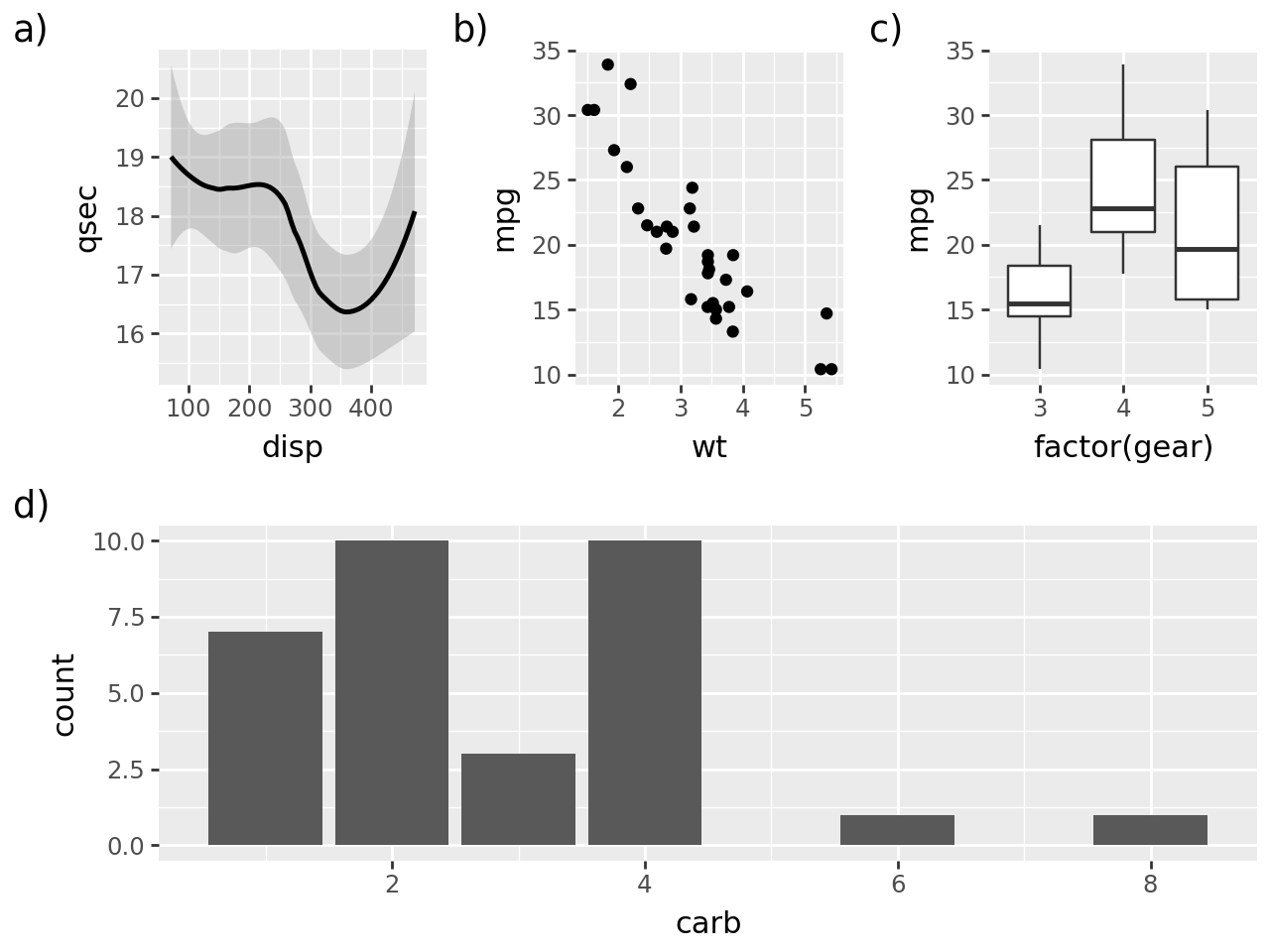
The position of each tag can be changed.
top_right = theme(plot_tag_position="topright")
top = theme(plot_tag_position="top")

p1_a = p1 + labs(tag="a)") + top_right
p2_b = p2 + labs(tag="b)") + top_right
p3_c = p3 + labs(tag="c)") + top_right
p4_d = p4 + labs(tag="d)") + top

(p1_a | p2_b | p3_c) / p4_d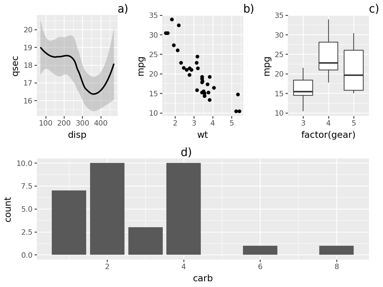
You can also set the location to one of margin (the default), panel, plot.
panel_top_right = theme(
    plot_tag_position="topright",
    plot_tag_location="panel",
    plot_tag=element_text(color="brown", margin={"t": 2, "r": 2})
)

p1_a = p1 + labs(tag="a)") + panel_top_right
p2_b = p2 + labs(tag="b)") + panel_top_right
p3_c = p3 + labs(tag="c)") + panel_top_right
p4_d = p4 + labs(tag="d)") + panel_top_right

(p1_a | p2_b | p3_c) / p4_d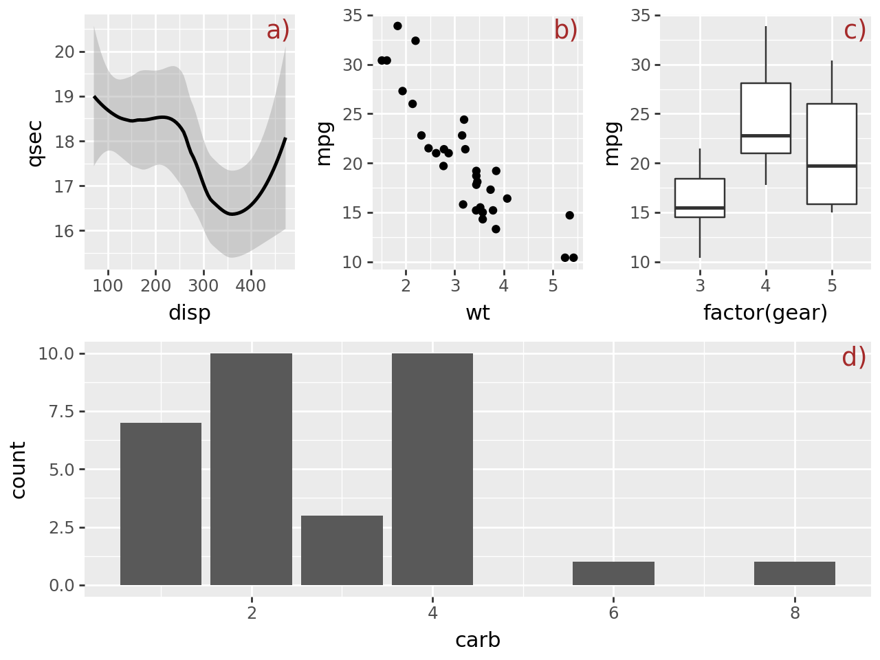
The valid positions for tags are topleft, top, topright, right, bottomright, bottom, bottomleft, left or a tuple[float, float].
Save
Use the save method to save the composition as an image e.g.
composition.save("plot.png")
composition.save("plot.png", dpi=200)
composition.save("plot.jpg")
composition.save("plot.svg")
composition.save("plot.pdf")Methods
| Name | Description |
|---|---|
| draw | Render the arranged plots |
| save | Save a composition as an image file |
| show | Display plot in the cells output |
draw(*, show=False)Render the arranged plots
Parameters
show : bool = False-
Whether to show the plot.
Returns
Figure-
Matplotlib figure
save(filename, format=None, dpi=None, **kwargs)Save a composition as an image file
Parameters
filename : str | Path | BytesIO-
File name to write the plot to. If not specified, a name
format : str | None = None-
Image format to use, automatically extract from file name extension.
dpi : int | None = None-
DPI to use for raster graphics. If None, defaults to using the
dpiof theme to the first plot. **kwargs-
These are ignored. Here to “softly” match the API of
ggplot.save().
show()Display plot in the cells output
This function is called for its side-effects.